Introduction
![]()
Chapters:
- Features
- Data Types
- Control Flow
- Functions
- Modules and Classes
- Ctypes and Misc
Python Features
Introduction:
This is an introduction to the structure and use of Python. Here you will learn how to use Python, basic functionality, and how to use the built-in Python documentation.
Topics Covered:
- Python Introduction
- Python Usage
- PyDocs
- Styling and PEP8
- Introduction to Objects
- Differences between version 2.x and 3.x
- Python Interpetor
- Running Python
To access the Python Features slides please click here
Lesson Objectives:
-
LO 1 Describe how to use Python from the command line (Proficiency Level: A)
-
LO 2 Explain the purpose and usage of elements and components of the Python programming language (Proficiency Level: B)
-
LO 3 Identify code written for Python 2 or Python 3 (Proficiency Level: B)
-
LO 4 Describe execution of Python from the command line (Proficiency Level: B)
-
LO 5 Use Python Documentation (PyDocs) (Proficiency Level: B)
-
LO 6 Apply Python standards (Proficiency Level: B)
- MSB 6.1 Interpret Python Enhancement Protocol 8 (PEP8) standards (Proficiency Level: B)
- MSB 6.2 Employ documentation of Python code (Proficiency Level: B)
- MSB 6.3 Describe the Python Library (Proficiency Level: B)
Performance Objectives (Proficiency Level: 3c)
-
Conditions: Given access to (references, tools, etc.):
- Access to specified remote virtual environment
- Student Guide and Lab Guide
- Student Notes
-
Performance/Behavior Tasks:
- Launch Python from the command line
-
Standard(s)
- Criteria: Demonstration: Correctable to 100% in class
- Evaluation: Students will have 4 hours to complete the timed evaluation consisting of both cognitive and performance components.
- Minimum passing score is 80%
Introduction to Python

Python is a high level programming language used for generic-purpose programming, created by Gudio van Rossum and released in 1991. Python's design philosophy focuses on code readability and syntax that allows programmers to express concepts in fewer lines of code. It's dynamic type system, auto memory management and standard library rest at it's core. Python is open source.
Why Python?
- High Level: strong abstraction of details from computer
- Interpreted: directly executes instructions and provides immediate feedback
- Readable: very easy to read, learn and understand
- Cross-Platform: runs almost anywhere
- Batteries-Included: deep functionality built into standard library
- General Language: can be used to do just about anything.
- Object Oriented Programming: allows code to be reused, encapsulated, maintained easier and organized cleaner.
Python Usage
- Prototyping
- Cross-platform scripts
- Automation and testing
- Vulnerability Research/Fuzzing
- Create/replicate pieces of software you do not otherwise have access to
- Web Development
- GUI/UX
- Gaming
- Etc.
PyDocs & PEP8
PyDoc(s)
- PyDocs is shorthand for Python Documentation and will be your go-to resource for everything Python. It is highly encouraged that you attempt to find the answer using PyDocs before asking an instructor or anyone else a question.
- Pydoc is a command that evokes the Python interpreter and utilizes the help() function to give you even more detail about a given object. You can also open up the Python interpreter and use help(object) replacing object with the object you want to look up.
- help() is a function that gives you a TON of data. For instance, object methods, module, important information, help, etc.
- Understanding how to use PyDocs, pydoc command and help() function is not only testable... but it's an essential piece in becoming proficient in Python.
2.7: https://docs.python.org/2.7/
3.x: https://docs.python.org/3/
Standard Library
The Python Standard Library contains all of the built in functionality of Python; and well, theres a lot of functionality included. The lectures will not even begin to scratch the surface of the Standard Library. With that said, you are encouraged to dive into the library and use whatever you can... whenever you can. You are not limited to just what I teach you. USE THE LIBRARY!
2.7: https://docs.python.org/2.7/library/index.html
3.x: https://docs.python.org/3.7/library/index.html
Pydocs Standard Library Requirments
You are required to look up each and everything we go over, using the PyDocs/pydoc/help(), throughout this course. Why? There are lots of functions and methods that can be applied to many different things. I will teach you many things as we go, but it's your responsiblity to ensure you know as much as possible per each topic we go over.
Styling and PEP8
PEP8 is shorthand for Python Enhancement Protocol 8. Think of this as the bible for Python; the dos and do-nots of formatting and styling. Below are some of the more important commandments.
- Python is whitespace sensitive! Unlike C, C++, Java, etc, Python does not use brackets. Instead, Python utilizes an indentation system.
- Spaces are preferred over tabs, you cannot mix. PEP8 commands 4 spaces per indention level (tab). Using editors with different tab settings may break code!
- To ensure you do not break your code... use spaces! (You can setup the tab button to output 4 spaces on most major text editors and IDEs)
PEP8: https://www.python.org/dev/peps/pep-0008/
Documenting Code:
Python brings many features we are already familiar with in other programming languages, but gives the user a bit more power in their documentation.
# This is a comment
"""This is a single line docstring"""
"""This is a multiline
comment
"""This is a multiline docstring

Notice the separation? Let's get into that and explain it.
"""
What is the difference between Docstrings and Comments?
- Docstrings are targeted towards people who don't need to know how the code works.
- Docstrings can be converted directly into actual documentation
- No implementation details unless they relate to the use
- Notice the gap in the multiline docstring?
- On a multiline docstring, the first line is a short description. This should only be one line.
- Second line is left blank to visually separate the summary from the rest of the description.
- The following lines are used for additional details
- Comments are used to explain what, why and how something is going on to other programmers. These are no different than C/C++ aside from syntax.
Exercise
- Take a moment to step through PEP8 and and learn the styling and formatting requirments
- Pay most attention to the basics:
- Indentation
- Maximum line length
- The entire comments section
- Ensure to include a docstring at the top of all of your labs that includes your:
- name
- project/lab
- date
- Ensure to include a docstring at the top of all of your labs that includes your:
- Naming Conventions
- Remember what else in contained within and return to PEP8 as we learn new concepts. You are expected to abide by PEP8 during the class.
Objects
Python has no unboxed or primitive types, no machine values. Instead, everything in Python is an Object! Objects involve an abstract way of thinking about programming. Down to the core, an object is just a struct; an encapsulation of variables and functions into a single entity. But on the surface, objects provide inheritance and other powerful uses.
- Inheritance simply means an object can be assigned to a variable or passed into a function for example.
- Unlike C, where an integer (for example) is a machine primitive… a single unstructured chunk of memory… a Python integer will be an object, a large block of structured memory, where different parts of that structure are used internally to the interpreter. Why does this matter? Thanks to everything being an object, our types have more features. Meaning... we can do more things to them. This also means they are larger than the machine primitve types we are used to.
Setting up your Python environment (lab 1A)
Please complete lab 1A setting up your Python environment.
Setup (Lab 1A)
Now that we learned the background behind Python, lets get to coding. Since Python is cross-platform, you can use whatever OS and text editor/IDE that you'd like. Below are my recommendations:
Recommended editors:
- Vim (terminal based: steep learning curve)
- Nano (terminal based)
- Visual Studio Code
- Sublime
- Atom
- Brackets
- Notepad++
Recommend against:
- Visual Studio
- Eclipse
- PyCharm
- EMacs
- etc
We flat out do not need a full fledged IDE for training. Python is easy to understand and type. We are going to focus on being independent and debugging with our own debugging code.
If your Python is out of date (2.7.15 & 3.7):
Python2
Ubuntu(debian based):
sudo apt install python
- The command for python2 in Ubuntu will be: python or python2
Windows:
- Install latest from https://www.python.org/downloads/windows/
- Ensure you check the PATH setup box during install
- The command for python2 in Windows will be: py -2
Python3
Ubuntu(debian based):
sudo apt install python3
- The command for python3.7 in Ubuntu will be: python3
-
Though that's a bit of a pain to write... so feel free to create an alias
-
The following are some suggested aliases:
alias py37=python3.7
alias python37=python3.7
-
Windows:
- Install latest from https://www.python.org/downloads/windows/
- Ensure you check the PATH setup box during install
- The command for python3 in Windows will be: py
Py2 vs Py3 Differences
Python 2 and 3 are similar but NOT COMPATIBLE! Python 3 does break compatibility. We will be focusing on Python 3.7 but will cover 2.7 along side the entire course. Here are just a few of the major differences:
Python 3 replaced Python 2's print statement with a print function(). While Python 2 will be happy as is or with parentheses... Python 3 will throw an error if the parentheses are not included.
Python 2
print 'Hello World!' # outputs: Hello World!
mystr = 'Goodbye World!' # Notice we didn't declare a type?

print mystr # outputs: Goodbye World!
print("This works too") # This works too!
Python 3
print("Hello World!") # Hello World!
mystr = 'Goodbye World!' # Again, no type declared. It's automatically determined.

print(mystr) # Goodbye World!
Integer Division
Python 2 treats numbers without a decimal as integers, whereas Python 3 will treat them as float if it applies. Python 2 Division with integers truncates the remainder! Setting one number as a real number will yield the correct result.
Python 2
print 3/2 # 1
print 3.0/2 # 1.5
Python 3
print (3/2) # 1.5
Other Major Differences
Unicode:
Python 2 has ASCII str() type, separate unicode() type.. but no byte() type.
Python 3 has Unicode (utf-8) str-ings and two byte classes: byte and bytearray.
We will cover both in later lectures.
Input() vs raw_input():
- Python 3 input() always stores userinput as str objects. This is good.
- Python 2 input() on the other hand fully evaluates the code the user gives it. This is dangerous! This gives the full power of Python to the user... and can be used in a malicious way. Instead, we use raw_input() in Python 2... which converts user input to a string.
There are more differences between the two major releases. It's encouraged to look up the differences for better understanding.
Running Python

Python Interpreter
There are a couple of ways to execute Python code. One way is through the Python Interpreter, which allows for on the fly code testing and sandboxing. The Python Interpreter uses a concept called REPL:
- Read the user input
- Some constructs like loops might be multiple lines
- Evaluate the input
- Attempt to perform the instruction
- Print: to the screen and
- Print any requested info or an error with stack trace
- Loop:
- Print the next user prompt or loop until evalution complete
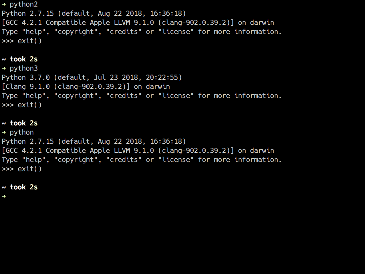
The Python Interpreter can be launched from the command prompt or terminal using the following commands:
Linux & OS X
- python2 or python generally opens up Python 2
- python3 generally opens up Python 3 (will open an out dated Python 3 one some distros)
- python3.7 opens up Python 3.7 currently on Fedora
- This is all dependent on a number of factors
- You can create aliases if you wish
Windows
- py -2 generally opens up Python 2
- py -3 or py generally opens up Python 3
- Again, this is all dependent on a number of factors
Additional Commands/Info
- exit() or shortcut crtl-D to exit the Python Interpreter.
- Typing simply a variable or expression will yield a printed output
# >>> represents the interpreter asking for a command.

>>> x = 100
>>> x
100
>>> x + 5
105
>>> x
100
-
Conditionals can be checked and loops can be executed. Be sure to provide indentation. This can be done via pressing the space bar 2 or 4 times per line or pressing tab.

Python Source Files
The other way to run Python code is using source files with the extension of .py. Python does not require compilation on the user's end. Executing .py source code is similar to starting the Interpreter.
Be sure to:
- Use appropiate bash commands for the source code's Python version
- Include filename and extension after bash command
- Include any arguments after filename and extension.
- We will go over ways to execute multiple files later in the course.
$ ls
file.txt    fileIO.py    hello_world.py    hello_world_3.py

$ python hello_world.py
Hello World!

$ python3 hello_world_3.py
Hello World for Python 3!
Data Types
Introduction:
Python uses several data types to store different variables as that all have different functionality. In this lesson you will go over the use and structure of the different data types.
Topics Covered:
- Variables
- Numbers
- Strings
- Lists
- Bytes and Bytearray
- Tuples
- Range
- Buffer
- Dictionaries
- Sets
- Conversion Functions
To access the Data Types slides please click here
Lesson Objectives:
-
LO 1 Describe tuples (Proficiency Level: B)
- MSB 1.1 Describe the purpose of tuples (Proficiency Level: B)
- MSB 1.2 Describe the properties of tuples (Proficiency Level: B)
-
LO 2 Discuss the use of the range() function in Python3
-
LO 3 Describe a string (Proficiency Level: B)
- MSB 3.1 Distinguish between the default string encoding in Python2 vs Python3 (Proficiency Level: B)
- MSB 3.2 Describe the options for string variable assignment (Proficiency Level: B)
- MSB 3.3 Identify string prefixes (Proficiency Level: B)
-
LO 4 Describe basic string methods (Proficiency Level: B)
-
LO 5 Comprehend dictionaries in Python (Proficiency Level: C)
- MSB 5.1 Describe the syntax to create a dictionary (Proficiency Level: B)
- MSB 5.2 Describe the syntax to access items in a dictionary (Proficiency Level: B)
- MSB 5.3 Describe the syntax to add, update and delete items in a dictionary (Proficiency Level: B)
- MSB 5.4 Describe the syntax to create and access multi-dimensional dictionaries (Proficiency Level: B)
-
LO 6 Comprehend sets Python (Proficiency Level: A)
- MSB 6.1 Describe the syntax to create a set (Proficiency Level: B)
- MSB 6.2 Describe the syntax to access items in a set (Proficiency Level: B)
- MSB 6.3 Describe the syntax to add and delete items in a set (Proficiency Level: B)
-
LO 7 Comprehend frozensets in Python (Proficiency Level: A)
-
LO 8 Differentiate operations that can be done to a set but not a frozenset in Python (Proficiency Level: A)
-
LO 9 Employ variables in Python (Proficiency Level: C)
- MSB 9.1 Describe the purpose of variables (Proficiency Level: B)
- MSB 9.2 Describe the syntax to determine data type of a variable (Proficiency Level: B)
- MSB 9.3 Describe the syntax to assign a variable (Proficiency Level: B)
-
LO 10 Apply the concept of mutability (Proficiency Level: B)
- MSB 10.1 Describe mutability (Proficiency Level: B)
- MSB 10.2 Identify the mutability of specific data types in Python (Proficiency Level: B)
-
LO 11 Distinguish between different number prefixes (Proficiency Level: B)
-
LO 12 Distinguish between different number types (Proficiency Level: B)
-
LO 13 Describe the Boolean data type (Proficiency Level: B)
-
LO 14 Employ arithmetic operators (Proficiency Level: C)
- MSB 14.1 Differentiate arithmetic operators (Proficiency Level: C)
- MSB 14.2 Given a scenario predict the resulting type of a math operation with different operand types (Proficiency Level: C)
- MSB 14.3 Differentiate bitwise operators (Proficiency Level: B)
- MSB 14.4 Describe the order of operations (Proficiency Level: B)
-
LO 15 Employ type conversion (Proficiency Level: C)
-
LO 16 Comprehend lists in Python (Proficiency Level: B)
- MSB 16.1 Describe the syntax to slice a list (Proficiency Level: B)
- MSB 16.2 Describe the syntax to retrieve/modify/delete an element of a list (Proficiency Level: B)
- MSB 16.3 Describe the syntax to combine a list (Proficiency Level: B)
- MSB 16.4 Comprehend multidimensional lists (Proficiency Level: B)
-
LO 17 Comprehend map, filter and reduce in Python (Proficiency Level: B)
Performance Objectives (Proficiency Level: 3c)
-
Conditions: Given access to (references, tools, etc.):
- Access to specified remote virtual environment
- Student Guide and Lab Guide
- Student Notes
-
Performance/Behavior Tasks:
- Store specified data in a tuple.
- Create a program using strings and string methods
- Utilize string methods to manipulate strings
- Store user input as a string
- Use the Python interpreter to identify the data type
- Use arithmetic operators to modify Python program functionality
- Use bitwise operators to modify Python program functionality
- Use type conversion to modify Python program functionality
- Use Python to create, access and manipulate a list
- Use Python to create, access and manipulate a Multi-dimensional list
-
Standard(s)
- Criteria: Demonstration: Correctable to 100% in class
- Evaluation: Students will have 4 hours to complete the timed evaluation consisting of both cognitive and performance components.
- Minimum passing score is 80%
Variables

EVERYTHING IN PYTHON IS AN OBJECT!
This is the single, most important thing taught in Python. The sooner you have an understanding of Python Objects, the quicker everything else falls into place. Objects are pieces of code that are designed to be interchangeable and thus reused, but more on this later.
Data types are dynamic based on the variable stored. To check type, use:
type(var)
# python2
x = 10
type(x)
# output: <type 'int'>

# python3
# output: <class 'int'>
Notice the output is <class 'int'> or <type 'int'>.... Type and class are interchangeable for our purposes. There was a time when they wern't. Once again, everything in Python is an object! We will go over type() more in meta-classes.
Multiple assignment
Multiple assignment is allowed and types can be the same or different:
# All == 100
a = b = c = 100

# Will only reassign variable c
c = 200

print ('a = {} b = {} c = {}'.format(a, b, c))
# output: a = 100 b = 100 c = 200

# will change all three variables
a,b,c = 100, 'hello', {}
print ('a = {} b = {} c = {}'.format(a, b, c))
#output: a = 100 b = hello c = {}
Data Types
- Numbers
- int, long, float, complex
- Strings
- Lists
- Think array
- Tuples
- Think constant array
- Dictionaries
- Think associative array
Data Types: Immutable
Immutable objects are those that can't be changed without reassigning. Such as int or str. Mutable objects are those that can be changed. Such as list or dict. Below is a table with all types and their mutability.

Continue to Performance Lab: 2A
Lab 2A
Using the Python interpreter: find the type of the following variables. Feel free to experiement with other variables and such.
Type of:
- 10
- 10.5
- "10"
- "Hello!"
- ""
- ''
- True
- 0
- type
- object
- b"10101101"
- 0b10101101
- [1,2,3]
- (1,2,3)
- {1,2,3}
- {'one':1}
- 5j
Numbers
Prefixes
Prefixes convert types like binary, hex and octal into int.
- No prefix for decimal
- Prefix with 0b, b for binary (ex. 0b10 == 2)
- Prefix with 0x, x for hex (ex. 0xF == 15)
- Prefix with 0o, o for octal (ex. 0o100 == 64)
$ py -3
>>> 0b10
2

>>> 0xF
15

>>> 0o100
64

>>> x = 0xF
>>> type(x)
<class 'int'>

>>> x
15
Types
-
int (integer)
- Equivalent to C-Longs in Python 2 and non-limited in Python 3
-
Long
- Long integers of non-limited length. Exist only in Python 2
-
Float (decimal, hex, octal)
- Floating point numbers. Equivalent to C-Doubles
-
Complex
- suffix is j or J
- There are several built-in accessors and functions to act on complex numbers
- We will not be going over these
- Complex numbers, ex:
x = 1.5 + 5j
y = 2
z = x + y
print(z)
#Output: (3.5+5j)

z = z + 3j
print(z)
#Output: (3.5+8j)
Numbers are IMMUTABLE!
Numbers cannot be modified in place. Be sure to either reassign your current variable or assign the number to a new variable.
$ py -3

>>> x = 10
>>> print(x)
10

>>> x = 15
>>> print(x)
15

>>> x = x + 5
>>> print(x)
20

>>> x + 5
25

>>> print(x)
20
Bool (True or False)
Bools are a subclass of int. This was done around Python 2.2 to allow previous implementations of bools (0 and 1) to continue working… especially so with C code that utilizes Pylint_Check()
Truth Value Testing
- The following will evaluate to False:
- False
- zero numeric type- 0 0.0 0
- None
- empty sequence – ‘’ () []
- empty mapping- {}
- instances of user defined classes (will get into later)
- The following will evaluate to True: Everything else, not limited to but including–
- True, 1
- any number that is less than or greater than 0... but not 0
- non-empty sequence/mapping, etc
Operators
There are some more differences between Python and many other languages that need to be brought to light. Increment operators (x++, y--, etc) do not exist in Python. To increment in Python, you can use shorthand: a += 1, x -= 5, z *= 2, etc
| Operator | Description | Example | Result |
|---|---|---|---|
| + | Addition | 4 + 5 | 9 |
| - | Subtraction | 10 - 5 | 5 |
| * | Multiplication | 4 * 2 | 8 |
| / | Division* | 3 / 2 | Py2(1) Py3(1.5) |
| // | Floor Division | 3.0 // 1.0 | 1 (~int division) |
| % | Modulus (remainder) | 4 % 2 | 0 |
| ** | Exponentiation | 4 ** 2 | 16 |
*3.0 / 2 will return 1.5 for both Python 2 and Python 3
- We are already familiar with what modulus does... it gives us the remainder.
- Floor division on the other hand is the equivalent of dividing 2 whole numbers that should have a remainder... in Python 2.
- Remember, Python 2 will truncate the remainder unless you specify one of the types as float.
- Floor division will always take the floor... or the lowest number. It does not round up.
Bitwise Operators
- Ahh, the dreaded bitwise operators are back!
- Bitwise Operators directly manipulate bits. There really is no speed advantage to bitwise operators in Python. The main advantage of bitwise operators is for scripting, compression, encryption, communication over sockets (checksums, stop bits, control algorithms, etc).
| Operator | Description | Example | Result |
|---|---|---|---|
| & | Binary AND | 1 & 3 | 0001 & 0011 == 0001 (1) |
| | | Binary OR | 1 | 3 | 0001 | 0011 == 0011 (3) |
| ^ | Binary XOR | 1 ^ 3 | 0001 ^ 0011 == 0010 (2) |
| ~ | Binary Ones Complement | ~3 | ~00000011 == 11111100 |
| << | Binary Left Shift | 1 << 3 | 00000001 << 3 == 00001000 |
| >> | Binary Right Shift | 1 >> 3 | 00000001 >> 3 == 00000000 |
Order of Operations
| Operation | Precedence | Extra |
|---|---|---|
| () | 1 | Anything in brackets is first |
| ** | 2 | Exponentiation |
| -x, +x | 3 | N/A |
| *, /, %, // | 4 | Will evaluate left to right |
| +, - | 5 | Will Evaluate left to right |
| <, >, <=, >=, !=, == | 6 | Relational Operators |
| Logical Not | 7 | N/A |
| Logical And | 8 | N/A |
| Logical Or | 9 | N/A |
Type Conversion
# int(x, base)
## Returns x as 'base' integer. 'base' specifies base if x is string, otherwise opitional
### EXAMPLE 1
x = 10.5
int(x)
# output: 10
### EXAMPLE 2
y = "101101"
int(y, 2) # specifiy y as a base 2
# output: 45
#########################
# float(x)
## Returns x as a float
x = 30
float(x)
# output: 30.0
#########################
# complex(real, imag)
## Returns complex number, defaults for real/imag is 0
complex(2, -3)
# output: (2-3j)
complex(2, 3)
# output: (2+3j)
#########################
# chr(x)
## Returns string of one character for x as ASCII
x = 10
chr(x)
# output: '\n'
x = 10.5
chr(int(x)) # notice what we did here?
# output: '\n'
#########################
# ord(x)
## Returns ASCII value for x as string of one char
ord('\n') # notice what we did here?
# output: 10
#########################
# hex(x)
## Returns x as hex value
hex(10)
# output: '0xa'
## Notice how the output is a string, there is no hex type
#########################
# oct(x)
## Returns x as octal
oct(10)
# output: '012'
## Same thing here
#########################
# bin(x)
## Returns x as binary
bin(10)
# output: '0b1010'
## Same thing here
There are some differences between Python 2 and Python 3 numbers. The biggest difference being the removal of the Long Type in Python 3.
Continue to Performance Labs: 2B and 2C
Lab 2B & Lab2C
Lab 2B: Numbers
- Instructions: Modify lab2b.py and follow the comment instructions.
- BONUS: shorten the code!
Lab 2C: Tax Calculator
- Instructions: Write a program that calculates the total of an item, with taxes.
- Bonus: Add additional functionality
- Keep in mind that you have not learned Python formatting for print or user input.
- Simple/ugly printing is allowed here.
- Hard code the user input
Strings
Reference: Strings
What is a sequence object?
A sequence object is a container of items accessed via index. Text strings are technically sequence objects.
Sequence Object Types:
- String
- Lists
- Tuples
- Range Objects
Each of the above support built in functions and slicing.
Sequence Objects: Strings
Strings are immutable! They need to be reassigned. There are two independent types of strings:
- ASCII: Default strings for Python 2
- Unicode (UTF-8): Default strings for Python 3
To declare a string, use one of the following. There is no Pythonic way aside from keeping it as simple and clean as possible.
- 'single quotes'
- "double quotes"
- ""escaped" quotes"
- """triple quoted-multiline"""
- r""raw" strings"

String Prefixes
- u or U for Unicode
- r or R for raw string literal (ignores escape characters)
- b or B for byte… is ignored in Python 2 since str is bytes.
- A ‘u’ or ‘b’ prefix may be followed by a ‘r’ prefix.
Yes, this stuff is old school and not very Pythonic... but it can't be helped.
Difference between ASCII and Unicode (utf-8)
ASCII defines 128 characters, mapped 0-127. Unicode on the other hand defines less than 2^21 characters, mapped 0-2^21. It is worth noting that not all Unicode numbers are assigned yet. Unicode numbers 0-128 have the same meaning as ASCII values; but do not fit into one 8-bit block of memory like ASCII values do. Thus Unicode in Python 3 utilizes utf-8 which allows for the use of multiple 8-bit blocks of memory.
Byte String vs Data String
Byte Strings are simply just a sequence of bytes. In Python 2, bytes is an alias of str. In other words, they are used interchangeably. In Python 3 on the other hand, str is it's own type... utilizing Unicode (utf-8). Whereas the bytes type in Python 3 is still a bytes object in ASCII; an array of integers.
Python 2
>>> x = "I am a string"
>>> type(x)
<type 'str'>
>>> x
'I am a string'
>>> hex(ord(x[0]))
0x49
Python 3
>>> x = 'I am a string'.encode('ASCII')
>>> type(x)
<class 'bytes'>
>>> print(hex(x[0]))
0x49 # ASCII code for capital I
>>> x = b'I am a string' # Doing this in Python 2 makes no difference
>>> type(x)
<class 'bytes'>
Unicode Strings
Python 2
>>> x = u"I am a unicode string"
>>> type(x)
<type 'unicode'>
>>> y = unicode("Look at me! I’m a unicode string.")
>>> type(y)
<type 'unicode'>
# You can use ‘…’ quotes “…” quotes or “””…””” quotes
Python 3
>>> x = 'I am a unicode string'
>>> type(x)
<class 'str'>
# class str is unicode in Python 3 natively
# You can use ‘…’ quotes “…” quotes or “””…””” quotes
Slicing
Slicing allows you to grab a substring of a string. Python's indexing structure starts at 0. The only exception is when grabbing an element using a negative index. There is an example further below.
Grabbing a specific element
>>> x = "hello world"
>>> print(x[4]) # grabs 4th index
o
Grab a range of elements
>>> x = "hello world"
>>> print(x[4:9]) # grabs 4th index up until, but not including the 9th index.
o wor
Grabbing backwards from the last element
>>> x = "hello world"
>>> print(x[-3]) # grabs the 3rd to the last ELEMENT
r
- Slicing with negative values start at -1, not 0. So if we have a string (x = "test"... t= -4, e = -3 s = -2 t = -1)... Thus a -2 slice will grab the 's'.
- When slicing a range, you grab everything UPTO (not including) the second defined index number.
More String Manipulation
- Try the following
>>> my_string = "Hello World!"
>>> print(my_string[0])
H
>>> print(my_string[0:5])
Hello
>>> print(my_string[6:])
World!
>>> print(my_string[-6:]) # ???
>>> print(my_string[::2]) # ???
>>> print(my_string * 2) # ???
>>> print(my_string + my_string) # ???
What did you get? Try different operations to manipulate strings!
String Special Operators
| Operator | Description |
|---|---|
| + | Concatenation |
| * | Repetition |
| [] | Slice |
| [:] | Range Slice |
| in | Membership - returns true if a character exists |
| not in | Membership - returns true if a character does not exist |
| % | Format |
User Input
There are a few ways to capture user input in Python. The most common are raw_input() in Python 2 and input() in Python 3. It is important that you use raw_input() in Python 2... as input() has security vulnerabilities. In Python 3, input() takes user input as a string, no matter the input. On the other hand, input() in Python 2 will take user input as the type presented. This can lead to users implementing false bools and such.
Python 2
>>> name = raw_input("What is your name? ")
What is your name? <user input>
>>> name
<user input>
Python 3
>>> name = input("What is your name? ")
What is your name? <user input>
>>> name
<user input>
As you more than likely guessed, the user input is assigned to the variable name and stored as a string. From here, you can treat var name as any other regular string.
Useful String Methods
- string.upper() # Outputs string as uppercase
- string.lower() # Outputs string as lowercase
- len(string) # Outputs string length
- symbol.join(string/list) # Most commonly used to join list items, outputs string.
- string.split(symbol )# Most commonly used to split a string up into a list of items, outputs list.
>>> my_string = "Hello World!”"
>>> a = my_string.upper()
>>> print(a)
'HELLO WORLD!'
>>> a = my_string.lower()
>>> print(a)
'hello world!'
>>> a = len(my_string)
>>> print(a)
12
>>> a = my_string.split(" ")
['Hello', 'World!']
>>> print(my_string)
'Hello World!'
>>> my_string = "+".join(a)
>>> print(my_string)
'Hello+World!'
Changing a Character
>>> my_string = "Hello World!"
>>> my_string[1]
'e'
>>> my_string[1] = 'E'
What's the outcome? How does replace() work?
Join
join() combines sequential string elements by a specified _str _separator. If no separator is specified join will insert white space by default.
Syntax:
str.join(sequence)
Example:
s = "-";
seq = ("a", "b", "c"); # This is sequence of strings.
print(s.join( seq ))

#Output: a-b-c
Split
split() will breakup a string and add the data to a string array using a defined separator.
Syntax:
str.split(str="", num=string.count(str))

#str - any delimeter, by default it is space.
#num - number of lines minus one.
Example:
x = 'blue,red,green'
x.split(",")

['blue', 'red', 'green']
>>>

>>> a,b,c = x.split(",")

>>> a
'blue'

>>> b
'red'

>>> c
'green'
Additional Standard Library Functionality
- startswith, endswith
- find, rfind
- count
- isalnum
- strip
- capitalize
- title
- upper, lower
- swapcase
- center
- ljust, rjust
Continue to Performance Labs: 2D and 2E
Lab 2D & Lab2E
Lab 2D: Strings
Instructions:
Write a program that reverses a user inputted string then outputs the new string, in all uppercase letters.
Bonus: Add additional functionality, experiment with other string methods.
Lab 2E: Count Words
Instructions:
Write a program that takes a string as user input then counts the number of words in that sentence.
Bonus: Add additional functionality, experiment with other string methods.
ex: Output number of characters, number of uppercase letters, etc...
Lists
Reference: Lists
Lists are very similar to C arrays. Lists are mutable and nestable. They are not ordered! There is no variable length per se, aside from what the system itself can handle. In other words, lists are dynamically adjusted to fit their contents. Lists can be multidimensional and can contain elements of different types. You can create a list using [].
List example:
>>> my_list = ['Hello World', 15, True, 'w']
>>> nested_list = [['such', 'wow'], 5, [False, '15']]
Slicing Lists
Much like strings, you can slice lists. There are some differences though. Slicing only one element will return a substring. Whereas slicing a range of elements will return another list.
Slicing One Element:
>>> my_list = ['apple', 'orange', 'cherry', 'strawberry']
>>> my_list[3]
'strawberry'
>>> type(my_list[3])
<class 'str'>
>>> nested_list = [['apple', 'orange'], ['onion', 'pepper']]
>>> nested_list[3] # ???
Slicing Multiple Elements
>>> my_list[0:2]
['apple', 'orange', 'cherry'] # outputs list
>>> type(my_list[0:2])
<class 'list'>
>>> nested_list[0][1]
'orange'
>>> nested_list[0][0:2]
['apple', 'orange']
>>> nested_list[0:2][1] # ???
Indexing Lists
index() will output the index (starting at 0) of an element that matches the index() argument. index() looks for strict matches. Overall, this is useful for finding the index of a specific item. For example:
>>> my_list = ['Hello World', 15, True, 'w']
>>> my_list.index(15)
1
>>> my_list.index('Hello')
Traceback (most recent call last):………
# index method looks for strict matches, ValueError: 'Hello' is not in list
# useful for finding index of a specific item
In/not in Operator
Works just like index().
>>> True in my_list
True
>>> 'Hello' in my_list
False
>>> 20 not in my_list
True
Modifying Lists
Remember, lists are MUTABLE! This simply means we can modify it in place via appending, removing, combining, etc.
Updating Lists:
- append()
- Adds on to the end of the list
- insert(i,x)
- Inserts object x into the list at offset index i)
- sort, sorted()
- Sorts list alphabetically
- Both accept a reverse parameter with a Boolean value
- Both also accept a key parameter that specifies a function to be called on each list element prior to making comparisons.
Example:
>>> my_list = [1,2,3,4,5]
>>> my_list.append(6)
[1, 2, 3, 4, 5, 6]
>>> my_list[0] = 99
>>> my_list
[99, 2, 3, 4, 5, 6]
>>> my_list.insert(0, 1)
>>> my_list
[1, 99, 2, 3, 4, 5, 6]
>>> messy_list = [2,1,4,5,3,5,100,222,44]
>>> sorted(messy_list)
# ??????
>>> print(messy_list)
>>> messy_list.sort()
# ??????
>>> print(messy_list)
>>> messy_list.sort(reverse=True)
>>> messy_list
# ??????
>>> print(messy_list)
Combining Lists:
- extend()
- concatenates the first list with another list or iterable.
- +=
- also concatenates the first list with another list or iterable.
- Example:
>>> rally_cars = ['Subaru', 'Ford’]
>>> rally_cars.extend(['Mini', 'Audi'])
>>> rally_cars
['Subaru', 'Ford', 'Mini', 'Audi']
>>> rally_cars += ['Peugeot', 'MG Metro']
>>> rally_cars
['Subaru', 'Ford', 'Mini', 'Audi', 'Peugeot', 'MG Metro']
Removing List Elements:
- list.remove(x)
- Removes the first value that matches x.
- del list[x]
- Removes a specific index.
- list.pop(x)
- Removes the specific index and returns the removed element.
Example:
# remove()
>>> my_list = [1,2,3,3,4,5]
>>> my_list.remove(3)
>>> my_list
[1, 2, 3, 4, 5]
# del
>>> del my_list[2]
>>> my_list
[1, 2, 4, 5]
# pop()
>>> my_list.pop(1)
2 # value popped
>>> my_list
[1, 4, 5]
Map, Filter, Reduce:
Map() applies a function to all the items in an input_list.
map(function_to_apply, list_of_inputs)
Example:
items = [1, 2, 3, 4, 5]
squared = []
for i in items:
    squared.append(i**2)
Map() allows us to implement this in a much simpler way.
items = [1, 2, 3, 4, 5]
squared = list(map(lambda x: x**2, items))
Don't fret over what lambda's are just yet. Just know they are condensed functions for now
def multiply(x):
    return (x*x)
def add(x):
    return (x+x)

funcs = [multiply, add]
for i in range(5):
    value = list(map(lambda x: x(i), funcs))
    print(value)

# Output:
# [0, 0]
# [1, 2]
# [4, 4]
# [9, 6]
# [16, 8]
Filter() - creates a list of elements for which a function returns true.
number_list = range(-5, 5)
less_than_zero = list(filter(lambda x: x < 0, number_list))
print(less_than_zero)

# Output: [-5, -4, -3, -2, -1]
The filter resembles a for loop but it is a builtin function and faster.
Reduce()- performs some computation on a list and returns the result. It applies a rolling computation to sequential pairs of values in a list.
Example: If you wanted to compute the product of a list of integers.
product = 1
list = [1, 2, 3, 4]
for num in list:
    product = product * num

# product = 24
Using reduce:
from functools import reduce # we will cover this later

product = reduce((lambda x, y: x * y), [1, 2, 3, 4])

# Output: 24
Continue to Performance Lab: 2F
Lab 2F
- Instructions:
- Write a program that will be able to check if two words (strings) are anagrams.
- An anagram is a word or phrase formed by rearranging the letters of a different word or phrase
- The program should include:
- All proper comments
- Needed docstrings
- User input (only expecting one user input due to not having gone over loops yet)
Bytes and Bytearray
Bytes()
It's worth re-mentioning that Python 2 and Python 3 have differences when it comes to bytes and strings. Python 2 strings are bytes naturally whereas Python 3 is unicode and needs to be defined as bytes when you want to use bytes type. Here are a couple ways to turn Python 3 strings and such.. into bytes. This functionality is backwards compatible with Python 2. It's highly recommended you define Python 2 strings the same way if you are going to be modifying the bytes. Even though it doesn't do anything in Python 2... it will make the job of refactoring code easier, if you had to up Python version to 3.x.
# Method 1 (shortest)
>>> x = b'hello world'
>>> print(x[1])
101 # ASCII dec value

# Method 2 (clean)
>>> x = 'hello world'
>>> y = bytes(x, 'ascii')
>>> print(y)
b'hello world'
>>> print(y[1])
101 # ASCII dec value

# python 2
>>> x = 'hello world'
>>> print ord(x[1])
# ord is the inverse of chr()... returns int representing the unicode code point of the argument
101 # Unicode dec value
This can go both ways. We can convert these integer representations back into Unicode or ASCII strings.
# Python 2 back to ascii string
>>> x = ord('e')
>>> x
101
>>> y = chr(x)
>>> y
'e'
# convert y into a unicode string (this only works in Python 2 because unicode is default in Python 3)
>>> y = unichr(x)
>>> y
u'e'

# Python 3 back to native unicode string
>>> x = ord('e')
>>> x
101
>>> y = chr(x)
>>> y
'e'
# y is now a unicode string... but how do we turn it into a byte/ascii string?
>>> y = bytes(y, 'ascii')
>>> y
b'e'
# Now y is a python 2 str type... bytes/ascii
Bytearray()
Bytearray() is a mutable sequence of integers in range of 0 <= x < 256; available in Python 2.6 and later. Byte Arrays are useful when you need to modify individual bytes in a sequence. Since bytearray() takes in a byte/ASCII string... there is a difference in how we must implement this function between Python 2 and 3.
Python 2
Python 2 strings, as noted above, are already byte/ascii strings. So all we have to do is pass it through as is. But remember, it's good practice to declare bytes; even in Python 2. (For this example, I will declare it for demonstration)
>>> x = "I am a string"
>>> b = bytearray()
>>> b.extend(x)
# This was done on purpose to show it is mutable
# You can pass the str directly into the bytearray() function to cut 2 lines
>>> b
bytearray(b'I am a string')
>>> b[2]
97 # decimal for 'a' char
>>> b[2] = 85 # Modifying a byte
>>> b
bytearray(b'I Um a string') # notice b did change without reassignment
Python 3
Python 3 strings on the other hand need to be converted before you can pass them as an argument into bytearray().
>>> b = bytearray(b"I am a string")
>>> b
bytearray(b'I am a string')
>>> b[2]
97 # decimal for 'a' char
>>> b[2] = 85
b
bytearray(b'I Um a string')
Continue to Performance Lab 2G
Lab 2G
- Follow the instructions on lab2g.py
Tuples, range & buffer
Tuples
Tuples are very similar to lists. The major difference is that tuples are IMMUTABLE! So just like strings and numbers, you cannot modify it's contents without reassigning. This also means that the length of tuples are set in stone. Parentheses (round brackets like these) are commonly used to declare tuples. There is a special type of tuple called a singleton. This is a tuple of one item and is denoted as singletonTuple = ('hello',). Don't be confused, this is not the same as a singleton design pattern, the naming convention of this type of tuple is derived from the mathematical usage of the word singleton, meaning one item in the set. You can declare tuples by just using commas.
# common method to declare tuples
>>> someTuple = (1,2,3,4,5)

# alternative method
>>> neatTuple = 1,2,3,4,5

>>> print neatTuple
(1, 2, 3, 4, 5)

#singleton Tuple
>>> singletonTuple = (1,)
# alternative method
>>> singletonAlternate = 1,


# What does the below do?
>>> del someTuple[2]
Why Use Tuples?
Tuples are still sequence objects. You can still:
- Implement all common sequence operations
- Slice
- Index
**Useful for:**
- Returning multiple results from functions
- Since they are immutable, they can be used as keys for a dictionary.
range()
Python 3's range() is essentially a combination of Python 2's range() and xrange() so luckily in Python 3 we only need to worry about using range(). We will mention xrange() so you have some exposure to it and are aware of its existence.
range() represents an immutable iterable object that always takes the small and same amount of memory irrespective of the size of range because it only stores start, stop, and step values and calculates values as needed.
Syntax
range(stop) range(start, stop,[ step])
start: Required when full syntax is used. An integer specifying start value for the range.
stop: Required. The boundary value for the range.
step: Optional. Step value.
>>> range(4)
range(0,4)

# if we want to see what is contained within our range
>>> list(range(4))
[0, 1, 2, 3]

>>> list(range(2,6))
[2, 3, 4, 5]

>>> list(range(0,50,5))
[0, 5, 10, 15, 20, 25, 30, 35, 40, 45]

>>> list(range(4,12,3))
# ???

>>> list(range(0,-10,-2))
# ???
We will cover range() more in depth and use it a lot more when we get to loops.
xrange()
xrange() is from Python 2 and is similar to range(), returns xrange object (sequence object) instead of list. Intended to be a simple, efficient (uses less resources due to one-at-time loading method vs loading all increments) and a fast way to iterate through a range. In most cases, xrange() will be the way to go. The only time you should use range() is when you are going to be iterating over the list multiple times. This is because xrange() will use more processing power over the length of the repeated iteration vs range... which will return a list and that list will stay and can be referenced whenever.
>>> for i in xrange(10):
>>>    print i
0
1
2
3
4
5
6
7
8
9

# Only even numbers
>>> for i in xrange(2, 10, 2):
>>>     print i
2
4
6
8

# Negative numbers
>>> for i in xrange(-1, -10, -1):
>>>     print i
-1
-2
-3
-4
-5
-6
-7
-8
-9
Buffer (memoryview)
Buffer (memoryview) is useful if you don’t want to or can’t hold multiple copies of data in memory. It can also be lightning fast since it's not copying the data. Buffer (or memoryview) essentially expose (by reference) raw byte arrays to other Python objects. That means the argument passed must be in bytes (ints representing bytes).
# Python 2
>>> x = b'100'
>>> buffer(x)
<read-only buffer for 0x10b1acc60, size -1, offset 0 at 0x10b1a9930>

# Python 3
>>> x = b'100'
>>> memoryview(x)
<memory at 0x1040b1948>
Practical Example
Below is a great example displaying how much resources and time buffer(memoryview) can save you. Copy, paste and run the code yourself. The first set of prints will be normal... the second will be using memoryview. Notice the amount of time it takes to complete each set of operations in bytes vs memoryview. While that may seem small... when more data is being manipulated, the time increases exponentially. A quick example can be found by running the same code below, but moving the prints into the while loops.
import time
for n in (100000, 200000, 300000, 400000):
    data = 'x'*n                            # set data = 'x'*n (if n were 5, xxxxxx)
    start = time.time()                     # start a timer
    b = data                                # set b = data
    while b:                                # remove one x and reasign to b, continue until 0
        b = b[1:]
    print 'bytes', n, time.time()-start     # stop time, print out time it took to do operation


# Same thing here, except we use memoryview instead
for n in (100000, 200000, 300000, 400000):
    data = 'x'*n
    start = time.time()
    b = memoryview(data)
    while b:
        b = b[1:]
    print 'memoryview', n, time.time()-start
Dictionaries and Sets
Mapping Types
Dictionary
Dictionaries are mutable objects and consist of key-value mappings. (ex: {key: ‘value’, key: ‘value’} ). They are initialized using the curly-brackets {}. Dictionaries are not ordered and support all value types.
>>> my_dict = {} # create empty dictionary
>>> my_dict['one'] = 1 # add item to the dictionary
>>> print my_dict
{'one': 1}
# OR
>>> my_dict = {'one' : 1} #create a dictionary with an item
>>> print my_dict
{'one': 1}
>>> my_dict['two'] = 2 # add item to the dictionary
>>> print my_dict
{'one': 1, 'two': 2}
# Grabbing by key
>>> new_dict = {'key1':'value1','key2':'value2','key3':'value3'}
>>> print new_dict['key2']
'value2'
Multi-Dimensional Dictionaries
Just like lists... Dictionaries can be nested as well to create a multi-dimensional dictionary.
# Dict -> Dict
>>> my_dict = {'key1':{'nestedkey1':{'subnestedkey1':'subnestedValue'}}}
>>> print my_dict
{'key1':{'nestedkey1':{'subnestedkey1':'subnestedValue'}}}

# Grab key 1's value
>>> print my_dict['key1']
{'nestedkey1': {'subnestedkey1': 'subnestedValue'}}

# Grab nested key 1's value
>>> print my_dict['key1']['nestedkey1']
{'subnestedkey1': 'subnestedValue'}

# Grab subnested key 1's value
>>> print my_dict['key1']['nestedkey1']['subnestedkey1']
subnestedValue
Common Dictionary Operations
>>> d[i] = y # value of I is replaced by y
>>> d.keys() # grabs all keys
>>> d.values() # grabs all values
>>> d.clear() # removes all items
>>> d.copy() # creates a shallow copy of dict_x
>>> d.fromkeys(S[,v]) # new dict from key, values
>>> d.get(k[,v]) # returns dict_x[k] or v
>>> d.items() # list of tuples of (key,value) pairs
>>> d.iteritems() # iterator over (key,value) items
>>> d.iterkeys() # iterator over keys of d
>>> d.itervalues() # iterator over values of d
>>> d.pop(k[,v]) # remove/return specified (key,value)
>>> d.popitem() # remove/return arbitrary (key,value)
>>> d.update(E, **F) # update d with (key,values) from E
Set and Frozenset
A set is an unordered collection of unique elements. Sets are mutable but contain no hash value-- so they can't be used as dict keys or as an element of another set.
>>> new_set = set() # create an empty set
>>> new_set = {0, 1, 1, 1, 2, 3, 4}
>>> new_set
{0, 1, 2, 3, 4}
>>> new_set.add(5) # Add new key to set
>>> new_set
{0, 1, 2, 3, 4, 5}
>>> x_set = set("This is a set")
>>> x_set
{'s', 't', 'e', 'h', 'I', ' ', 'T', 'a'}
>>> another_set = set(['Ford', 'Chevy', 'Dodge', 105, 555])
{'Chevy', 105, 155, 'Ford', 'Dodge'} # many ways to create set
Frozenset
Frozensets are identical to sets aside from the fact that they are immutable. Since frozensets are immutable, they are hashable as well. So they can be used as a dict key or element of another set.
>>> new_set = frozenset([1,2,2,2,3,4])# create an frozenset
>>> new_set
frozenset({1, 2, 3, 4})
>>> new_set.add(5)
.......AttributeError: ‘frozenset’ object has no attribute ‘add’
# Doesn't work since Frozenset is immutable
# Many… many ways to create frozenset as well.
Common Set Operations
Some do not apply to Frozenset.
>>> s.issubset(t) # test if elements in s are in t
>>> s.issuperset(t) # test if elements in t are in s
>>> s.union(t) # new set with elements of t and s
>>> s.intersection(t) # new set with common elements
>>> s.difference(t) # new set with elements in s but not t
>>> s.symmetric_difference # xor
>>> s.copy() # new shallow copy of s
>>> s.update(t) # return set s with elements from t
>>> s.intersection_update(t)
>>> s.difference_update(t)
>>> s.symmetric_difference_update(t)
>>> s.add(x) # add x to set s
>>> s.remove(x) # remove x from set s
>>> s.discard(x) # remove x from set s if present
>>> s.pop() # remove arbitrary item
>>> s.clear() #remove all elements from set a
Additional Functionality
Conversion Functions
Below are some functions to convert a variable to another type.
>>> int()
>>> long()
>>> float()
>>> complex()
>>> str()
>>> repr()
>>> eval()
>>> tuple()
>>> list()
>>> set()
>>> dict()
>>> frozenset()
>>> chr()
>>> unichr()
>>> ord()
>>> hex()
>>> oct()
>>> bin()
Import Sys
Sys is a large module from the Standard Library that contains very useful code and functionality. We will get into what modules are and how to import and such later in the course. For now, we are going to focus on one function from the module.
sys.getsizeof(object) --gets the size of the object passed in bytes. As you can imagine, this is going to be very helpful in streamlining your code.
Documentation:
Example:
>>> import sys
>>> x = 40
>>> sys.getsizeof(x)
12
Continue to Performance Lab: 2H
Lab 2H
Create a program that takes input of a group of students' names and grades... then sorts them based on highest to lowest grade. Then calculate and print the sorted list and the average for the class. (Hint: Use Dictionaries!)
Flow Control
Introduction:
This lesson will walk you through the control flow, which is the order your python scripts operate. Python uses the typical flow control statements.
Topics Covered:
To access the Control Flow slides please click here
Lesson Objectives:
-
LO 1 Comprehend if, elif, else statements in Python (Proficiency Level: B)
- MSB 1.1 Describe if, elif, else syntax (Proficiency Level: B)
- MSB 1.2 Given Python Code, predict the behavior of code involving if, elif, else syntax. (Proficiency Level: B)
-
LO 2 Comprehend While loops in Python (Proficiency Level: B)
- MSB 2.1 Describe While loop syntax (Proficiency Level: B)
- MSB 2.2 Describe using the while loop to repeat code execution. (Proficiency Level: B)
- MSB 2.3 Given Python Code, predict the outcome of a while loop. (Proficiency Level: B)
-
LO 3 Comprehend For loops in Python (Proficiency Level: B)
- MSB 3.1 Describe For loop syntax (Proficiency Level: B)
- MSB 3.2 Describe using the For loop to iterate through different data type elements. (Proficiency Level: B)
- MSB 3.3 Given Python Code, predict the outcome of a For loop. (Proficiency Level: B)
-
LO 4 Comprehend Python operators (Proficiency Level: B)
- MSB 4.1 Describe the purpose of membership operators (Proficiency Level: B)
- MSB 4.2 Describe the purpose of identity operators (Proficiency Level: B)
- MSB 4.3 Describe the purpose of boolean operators (Proficiency Level: B)
- MSB 4.4 Describe the purpose of assignment operators (Proficiency Level: B)
-
LO 5 Given a scenario, select the appropriate relational operator for the solution. (Proficiency Level: C)
-
LO 6 Given a code snippet containing operators, predict the outcome of the code. (Proficiency Level: C)
-
LO 7 Comprehend the purpose of the Break statement (Proficiency Level: B)
-
LO 8 Comprehend the purpose of the Continue statement (Proficiency Level: B)
-
LO 9 Given a code snippet, predict the behavior of a loop that contains a break/continue statement. (Proficiency Level: B)
Performance Objectives (Proficiency Level: 3c)
-
Conditions: Given access to (references, tools, etc.):
- Access to specified remote virtual environment
- Student Guide and Lab Guide
- Student Notes
-
Performance/Behavior Tasks:
- Control the execution of a program with conditional if, elif, else statements.
- Use a while loop to repeat code execution a specified number of times
- Iterate through Python object elements with a For loop
- Utilize assignment operators as part of a Python code solution.
- Utilize boolean operators as part of a Python code solution.
- Utilize membership operators as part of a Python code solution.
- Utilize identity operators as part of a Python code solution.
- Utilize break or continue statements to control code behavior in loops.
-
Standard(s)
- Criteria: Demonstration: Correctable to 100% in class
- Evaluation: Students will have 4 hours to complete the timed evaluation consisting of both cognitive and performance components.
- Minimum passing score is 80%
Operators
Comparison Operators
- x == y
- if x equals y, return True
- x != y
- if x is not y, return True
- x > y
- if x is greater than y, return True
- x < y
- if x is less than y, return True
- x >= y
- if x is greater or equal to y, return True
- x <= y
- if x is less or equal to y, return True
Example:
a=7
b=4

print('a > b is',a>b)

print('a < b is',a<b)

print('a == b is',a==b)

print('a != b is',a!=b)

print('a >= b is',a>=b)

print('a <= b is',a<=b)


#Output
a > b is True
a < b is False
a == b is False
a != b is True
a >= b is True
a <= b is False
Membership Operators
- in
- Evaluates to True if it finds a variable in the checked sequence
- not in
- Evaluates to True if it does not find a variable in the checked sequence
Identity Operators
- is
- Evaluates to True if variables on either side of the operator point to the same object
- is not
- Evaluates to True if the variables on either side of the operator does not point to the same object
Boolean Operators
- and
- Evaluates True if expressions on both sides of the operator are True.
- or
- Evaluates True if expressions on either side of the operator are True.
Examples:
# Example using bitwise operators
a=7
b=4

# Result: a and b is 4
print('a and b is',a and b)

# Result: a or b is 7
print('a or b is',a or b)

# Result: not a is False
print('not a is',not a)

#Output
a and b is 4
a or b is 7
not a is False


# Example using 'in' operator
list1=[1,2,3,4,5]
list2=[6,7,8,9]
for item in list1:
    if item in list2:
        print("overlapping")
else:
    print("not overlapping")

# Output: not overlapping


# Example of 'is' identity operator
x = 5
if (type(x) is int):
    print ("true")
else:
    print ("false")

# Output: true
Assignment Operators
| Operator | Example | Similar |
|---|---|---|
| = | x = 8 | x = 8 |
| += | x += 8 | x = x + 8 |
| -= | x -= 8 | x = x - 8 |
| *= | x *= 8 | x = x * 8 |
| /= | x /= 8 | x = x/8 |
| %= | x %= 8 | x = x%8 |
| **= | x **= 8 | x = x**8 |
| &= | x &= 8 | x = x & 8 |
| |= | x |= 8 | x = x|8 |
| ^= | x ^= 8 | x = x ^ 8 |
| <<= | x <<= 8 | x = x << 8 |
| >>= | x >>= 8 | x = x >> 8 |
I/O Print
Python print/print() is very powerful... taking styling from C string formating and adding some of it's own features; allowing for deeper functionality. Pull up PyDocs and reference Py2 and Py3 print, %, and formatting.
Note: Python2 and Python3 print statement/function automatically creates a newline. We can get around this if needed.
Python 2 Basic:
print "hello" # print statement only valid in Py2
print 1+1
print 'Hello' + 'world'
print('Hello' , 'World') # print function valid in both Py2 and Py3 (use this)

# Printing without newline, still has space seperating though
print "First statement ",
print "%s" % ("Second statement"),
print "Third statement"
# Output: 'First statement Second statement Third statement'
Python 3 Basic:
print("hello")
print(1+1)
print('Hello' + 'World')
print('Hello' , 'World')

# Printing without newline
print("First statement ", end=" ")
print("{}".format("Second statement"), end="")
print("Third statement")
# Output: 'First statement  Second statementThird statement'
% Formatting
% formatting follows C style and is being phased out. It is highly recommend to use .format()… but have practice with both!
# Basic Positional Formatting
print "%s World!" % "Hello"
'Hello World!'
# Basic Positional Formatting
print "%s %s!" % ("Hello", "World")
'Hello World!'
# Padding 10 left
print '%10s' % ('test',)
' test'
# Negative Padding (10 right)
print '%-10s %s' % ('test', 'next word')
'test next word'
# Truncating Long Strings
print '%.5s' % ('what in the world',)
'what '
# Truncating and padding
print '%10.5s' % ('what in the world',)
' what'
# Numbers
print '%d' % (50,)
50
# Floats
print '%f' % (3.123513423532432)
3.123513
# Padding numbers
print '%4d' % (50,)
50
# Padding Floating Points/precision
print '%06.2f' % (3.141592653589793,)
003.14
# Name Placeholders
things = {'car': 'BMW E30', 'motorcycle': 'Harley FXDX'}
print 'My fav car %(car)s and motorcycle %(motorcycle)s' % things
'My fav car BMW E30 and motorcycle Harley FXDX'
.format()
Format() is the latest formatting functionality. PEP8 highly encourages the use of .format() whenever possible. .format() includes most of the previous functionality with a ton of added functionality as well. Below is just SOME of the built in .format() functionality. Keep in mind, you can create custom functionality with .format(). Take a look at the docs and below and experiment!
# Basic Positional Formatting
print('{} {}!'.format('Hello', 'World'))
'Hello World!'
# Basic Positional Formatting
print("{!s} {!s}".format("Hello", "World"))
'Hello World!'
# Actual Positional Formatting
# EXCLUSIVE
print('{1} {0}!'.format('World', 'Hello'))
'Hello World!'
# Padding 10 left
print('{:>10}'.format('test'))
' test'
# Negative Padding 10 right
print('{:<10}'.format('test'))
'test '
# Changing Padding Character
# EXCLUSIVE
print('{:_>10}'.format('test'))
'______test'
# Center Align
# EXCLUSIVE
print('{:_^10}'.format('test'))
'___test___'
# Truncating Long Strings
print('{:.5}'.format('what in the world'))
'what '
# Truncating and padding
print('{:10.5}'.format('what in the world'))
' what'
# Numbers
print('{:d}'.format(50))
50
# Floats
print('{:f}'.format(3.123513423532432))
3.123513
# Padding numbers
print('{:4d}'.format(50))
50
# Padding Floating Points/precision
print('{:06.2f}'.format(3.141592653589793))
003.14
# Name Placeholders
things = {'car': 'BMW E30', 'motorcycle': 'Harley FXDX'}
print('My favorite car is a {car} and motorcycle {motorcycle}'.format(**things))
'My fav car BMW E30 and motorcycle Harley FXDX'
# Date and Time
# EXCLUSIVE
from datetime import datetime
print('{:%Y-%m-%d %H:%M}'.format(datetime(2017, 10, 17, 10, 45)))
2017-10-17 10:45
#Variables
nBalloons = 8
print("Sammy has {} balloons today!".format(nBalloons))
Output
Sammy has 8 balloons today!
sammy = "Sammy has {} balloons today!"
nBalloons = 8
print(sammy.format(nBalloons))
Output
Sammy has 8 balloons today!
| Format Symbol | Conversion |
|---|---|
| %c | character |
| %s | string conversion via str() prior to formatting |
| %i | signed decimal integer |
| %d | signed decimal integer |
| %u | unsigned decimal integer |
| %o | octal integer |
| %x | hexadecimal integer (lowercase letters) |
| %e | exponent notation |
| %f | floating point real number |
Continue to Performance Lab: 3A
Lab 3A

General
Create your own mad libs game asking the user for input to fill in the blanks. Print out using .format().
(Humor encouraged)
Background
"Mad Libs is a phrasal template word game where one player prompts others for a list of words to substitute for blanks in a story, before reading the – often comical or nonsensical – story aloud. The game is frequently played as a party game or as a pastime."
Requirments
- Adhere to PEP8 (Comments, formatting, style, etc)
- Create a handfull of pharses that require different numbers of inputs
- Prompt the user for input(s):
- Inputs can be done a number of ways...
- (SIMPLE) Ask user for input directly, tell them if the word(s) need to be a verb, noun, etc.
- (Moderate) Give the user a handful of choices per input to choose from.You will need to create a bank of verbs, nouns, etc for this.
- (Harder) Give the user cards based off the actual game. Allowing them to draw, etc following the rules. Allow them to only input those cards.
- (opitional) Implement basic user input checking:
- Check to ensure words are words, numbers are numbers (there are many ways to do this)
- Ensure symobls aren't used if they are not needed
- Check length
- etc
- Implement re-input if input is incorrect
- Inputs can be done a number of ways...
- Output the user inputs into the given pharse
- Use formatting to not only output the user inputs, but to create a UI within the terminal. Space out certain UI elements such as title of program, choices, menu deceration, etc.
I/O: Files
Reference: File Objects
Python offers a robust and insanely easy to use toolset to interact with files.
First, a file must be opened before it can be modified... this includes creating new files. We use the open() function to achieve this. The first argument passed is the file name; rather it exists or not. The second argument is the operation in which we would like to perform. ex read, write, overwrite, etc.
file = open("file.txt", 'r')
open() Operation Arguments
read
r -- Opens file for read only. File pointer is placed at start of file.
rb -- Opens a file for reading only in binary format. The file pointer is placed at the start of the file.
r+ -- Opens a file for both reading and writing. File pointer is placed at the start of the file.
rb+ -- Opens a file for both reading and writing in binary format. File pointer is placed at the start of the file.
write
w -- Opens a file for writing only. Overwrites the file if it exists. If the file does not exist, it creates a new one.
wb -- Opens a file for writing only in binary format. Overwrites the file if it exists. If it does not exist, it creates a new one.
w+ -- Opens a file for writing and reading. Overwrites the existing file if it exists. If it does not exist, it creates a new one.
wb+ -- Opens a file for writing and reading in binary format. Overwrites the existing file if it exists. If not, it creates a new one.
append
a -- Opens a file for appending. File pointer is at end of file if it exists. If the file does not exist, it creates a new one
ab -- Opens a file for appending in binary format. File pointer is at end of file if it exists. If not, it creates a new one.
a+ -- Opens a file for both appending and reading. If file exists, file pointer placed at end of file. If not, it creates a new one.
ab+ -- Opens a file for both appending and reading in binary format. Follows above file pointer and write rules.
Advantages of Using Binary Formatting
The advantages of using binary formatting primarily apply to Windows. Unlike Linux, where "everything is a file"... Windows treats binaries and files differently. Thus, reading binary in text mode in Windows will more than likely result in corrupted data. Passing a 'b' variant will mitigate this issue.
File Operations
Once the file is open, we can begin reading, adding or modifying the file's contents. Below are some of the methods to make that happen.
- f.write(str)
- write str to file
- f.writelines(str)
- write str to file
- f.read(sz)
- read size amount
- f.readline()
- read next line
- f.seek(offset)
- move file pointer to offset
- f.tell()
- current file position
- f.truncate(sz)
- truncate the files z bytes
- f.mode()
- returns the access mode used to open a file
- f.name()
- returns the name of a file
- f.close()
- close file handle...
- Just like other programming languages, we need to close the stream
- ALWAYS CLOSE THE FILE AS SOON AS YOU'RE FINISHED USING IT!!
f = open('file_name', 'a')
data = f.read()
print data

file.close()
Continue to Performance Lab: 3B
Lab 3B
Instructions
Instructions:
- You are provided with a text file that contains the best song lyrics in the world
- Problem is... the song lyrics are encrypted with a simple XOR.
- You will need to decrypt the lyrics
- The key is 27
- You have been provided with a decent chunk of the code with conditionals and loops already created...
- Feel free to create yours from scratch if you want a greater challenge.
- You will need to think outside the box. Remember what XOR is, the type of data it acts on, how much data, etc.
Requirements
- Adhere to PEP8 (Comments, formatting, style, etc)
- Follow instructions above
Link To Student Code
If, Elif, Else
Just like most other programming languages, Python includes the standard if, else-if, and else statements. The only difference is that Python's else-if statement is shortened to elif. The if statement checks for truth within a given condition. If the condition is false, the code within the if statement will not run. To counter this, you can use elif statements to check for further conditions. Finally we have the else statement which is a catch all if none of the previous statements evaluate to True.
Note: If even one statement in an if/elif is evaluated as true, all the remaining conditions will not be checked. Conditions are checked from top to bottom. Some situations call for multiple if statements, some work better with if/elif/else statements. Just keep in mind the order of the statements.
As mentioned in previous lectures, Python does not use brackets. So unlike C, Java, etc... Python uses indentation. To make this work for statements, loops, functions, etc... Python uses a colon ':' to declare the start of an indented block.
a = 100
if a > 100:
    print('a is greater than 100')
elif a < 100:
    print('a is less than 100')
else:
print('a is equal to 100')
Output:
a is equal to 100
Another Example:
What is the output?
for a in range(51):
    if a == 0:
        print("{} you can't divide by zero!".format(a))
    elif a % 10 == 0:
        print ('{} can be divided by 10!!!'.format(a))
    elif a % 2 == 0:
        print('{} is even!'.format(a))
    else:
        print('{} is odd!'.format(a))
Continue to Performance Lab 3C
Lab 3C

Instructions
Create a text-based game where the user is navigating through a "Fun" House. Prompt the user to make a decision and using if/elif/else statements, give them different outcomes based on their answers. Begin with an introduction to your fun house and prompt the user to choose between at least three different options. You can use nested if/elif/else statements to make the game more complex.
Requirments
- Adhere to PEP8 (Comments, formatting, style, etc)
- Utilize userinput
- Utilize proper formatting
- Utilize proper and clean if/elif/else statements
- Follow instructions above
Additional
- Take this a step further. Use some previous concepts. Here are some things you can do:
- Create a file that holds all of your prompts
- Store file prompts into a list, dict, etc
- Use if/elif/else statements to validate user input
- Use formatting to create UI elements and/or fancy prompts
- Use operators and user input to perform calculations based on prompts
- etc
Example:
print "Welcome to Fun House! Choose door 1, 2, or 3..."

input = raw_input("> ")

if input == "1":
    #<code>
    print"1"

elif input == "2":
    #<code>
    print "2"

elif input == "3":
    #<code>
    print "3"
else:
    print "Go home you're drunk."
While Loops
While loops, just like C and C++, loop through each iteration until either the condition is met or a break statement is called. Being that this is a loop... it is possible and rather easy to get stuck in an infinite loop. Keep in mind, you cannot use the x++ incrementer in Python.
count = 0
while count < 10:
    print('count: ' + str(count))
    count += 1
Output:
count: 0
count: 1
count: 2
count: 3
count: 4
count: 5
count: 6
count: 7
count: 8
count: 9
When using the while loop, a few factors will make a difference in the output... that could break your program if you don't pay attention. The value of the incrementing var, where the count increment is placed and the comparison operator are the three most common factors. Here are a few things to keep in mind:
- It's common practice to increment your var after the bulk of the code is executed (count += 1)
- With that said, setting the count equal to 0 will start the output at 0, 1 will start at 1... etc
- It's best practice to change the comparison operator rather than the 'increment to number'. For instance, count is currently set to increment until 10. Since the code increments after the print is executed... the last count printed is 9, even though the count really ends on 10. If you follow the above factors, changing the comparison operator to <= will result in an output that prints count: 10 without effecting code that relies on count.
While Else
Python allows for the use of a While-Else Statement. The while-else runs like a regular while loop except for the one iteration when the while loop becomes false. This results in the else statement being executed once!
count = 0
while count <= 10:
    print('count: {}'.format(count))
    count += 1
else:
    print('while loop executed... count is: {}'.format(count))
Output:
count: 0
count: 1
count: 2
count: 3
count: 4
count: 5
count: 6
count: 7
count: 8
count: 9
count: 10
while loop executed... count is: 11
This gives us a clearer look at how Python increments variables.
Continue to Performance Lab: 3D
Lab 3D
Instructions
- Write a program that prompts a user to input an integer and calculates the factorial of that number using a while loop.
Requirments
- Adhere to PEP8 (Comments, formatting, style, etc)
- Utilize userinput
- Utilize input validation
- Utilize proper formatting
- Utilize proper and clean loops and conditionals
- Follow instructions above
For Loops
For Loop in C:
char *my_string = "Python";
for (int i = 0; i < strlen(my_string); i++) {
    printf(%c\n", my_string[i]);
}
Python in C Style:
my_string = "Python"
for i in range(len(my_string)):
    print(my_string[i])
While the Python one certainly is shorter and looks cleaner... it's still not Pythonic for our use. Though, there will be times where range(len()) formula is useful... mostly when dealing with mutable types.
For Loop... Python Style
my_string = "Python"
for letter in my_string:
    print(letter)
So easy, a caveman can do it! But, how does this happen under the hood?
Remember Data Types chapter? Strings are iterable. The "in" operator simply calculates the count of my_string and iterates through it as var letter. The value of letter is my_string[i].
For Looping Dictionaries
One way to set up looping for a dictionary
#In python 2 use the method iteritems()
for key, value in dict.iteritems():
    pass
#In python 3 the method is now just items()
for key, value in dict.items():
    pass
Here is an example of how to do this
x = {'stu1':'James', 'stu2':'Bob', 'stu3':'Rengar'}

for stu_id, name in x.items():
    print("{}'s name is {}".format(stu_id, name))
Loops: Iterative vs Recursive
Iteration and recursion each involve a termination test: Iteration terminates when the loop-continuation condition fails; recursion terminates when a base case is recognized.
Recursion repeatedly invokes the mechanism, and consequently the overhead, of method calls. This can be expensive in both processor time and memory space. In almost all cases it is better to use iterative loops.
Iteration
When a loop repeatedly executes until the controlling condition becomes false.
Recursion
When a statement in a function calls itself repeatedly.
Continue to Performance Lab: 3E
Lab 3E
Instructions:
- Write a file that prints out the first 100 numbers in the Fibonacci sequence iteratively
- Revist this lab and create a Fibonacci recursive function
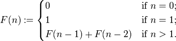
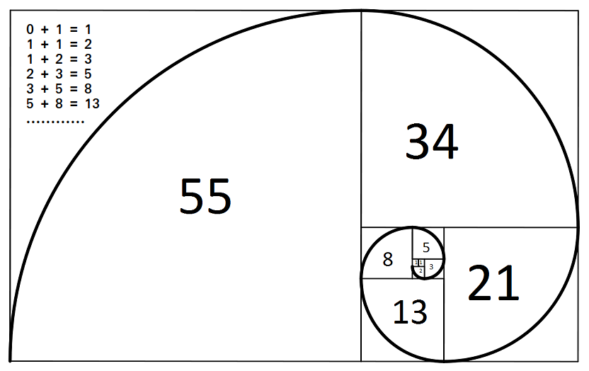
Requirments:
- Adhere to PEP8 (Comments, formatting, style, etc)
- Utilize proper formatting
- Utilize proper and clean loops and conditionals
- Follow instructions above
Additional:
- Some additional things you can do are:
- Utilize functions
- Create the recursive solution before going over ch04
- Utilize some Python modules or built in functionality
- Ask user for range of numbers to calculate
- Utilize functions
Break and Continue
If further examples are needed of how Break/Continue works, please reference PyDocs.
Break
The break statement simply breaks out of the innermost enclosing loop.
for i in range(1, 101):
    if i == 10:
        print("WE BROKE IT!")
        break
    print(i)
Output:
1
2
3
4
5
6
7
8
9
WE BROKE IT!
Continue
The continue statement continues with the next iteration of the loop.
for i in range(1, 100):
if i % 2 == 0:
print("{} is an even number!".format(i))
continue #prevents second print from running
print("{} is an odd number!".format(i))
Output:
1 is an odd number!
2 is an even number!
3 is an odd number!
4 is an even number!
5 is an odd number!
6 is an even number!
7 is an odd number!
8 is an even number!
9 is an odd number!
10 is an even number!
11 is an odd number!
12 is an even number!
13 is an odd number!
14 is an even number!
15 is an odd number!
16 is an even number!
17 is an odd number!
18 is an even number!
19 is an odd number!
20 is an even number!
....
Notice how the second print is skipped entirely for even numbers!
Continue to Performance Lab: 3F
Lab 3F
Instructions:
- Iterate through a loop 100 times… printing “Fizz” for any number divisable by 3 and “Buzz” for any number divisable by 5. If the number is divisable by both… print “FizzBuzz”. All other numbers… print the number.
Requirments:
- Adhere to PEP8 (Comments, formatting, style, etc)
- Utilize proper formatting
- Utilize proper and clean loops and conditionals
- Follow instructions above
Additional:
- Create two versions:
- One version which is as short as possible
- Another version which is as drawn out and creative as possible
Example Output:
1
2
Fizz
4
Buzz
Fizz
7
…
14
FizzBuzz
…
Functions
Introduction:
This lesson takes a look into the creation and use of Python functions.
Topics Covered:
- Scope
- User Functions
- Parameters and Arguments
- Commandline Arguments
- Returning
- Pass By Reference
- Lambda Functions
- List Comprehension
- Closures
- Iterators
- Generators
To access the Functions slides please click here
Lesson Objectives:
-
LO 1 Understand the scope of a declared variable in Python. (Proficiency Level: B)
-
LO 2 Describe the purpose and use of iterators in Python (Proficiency Level: B)
-
LO 3 Describe the purpose and use of generators in Python (Proficiency Level: B)
-
LO 4 Understand how functions are created and implemented in Python. (Proficiency Level: B)
- MSB 4.1 Understand the purpose of the return statement in Python. (Proficiency Level: B)
- MSB 4.2 Understand the purpose of parameters for a function in Python. (Proficiency Level: B)
- MSB 4.3 Understand how return values are used in a function in Python. (Proficiency Level: B)
- MSB 4.4 Understand how to implement a function that returns multiple values in Python. (Proficiency Level: B)
-
LO 5 Describe the purpose and use of lambda functions in Python. (Proficiency Level: B)
Performance Objectives (Proficiency Level: 3c)
-
Conditions: Given access to (references, tools, etc.):
- Access to specified remote virtual environment
- Student Guide and Lab Guide
- Student Notes
-
Performance/Behavior Tasks:
- Write a program to parse command line arguments in Python.
- Write a program to return multiples values in Python.
- Write a program to receive input parameters in Python.
- Create and implement functions to meet a requirement in Python.
-
Standard(s)
- Criteria: Demonstration: Correctable to 100% in class
- Evaluation: Students will have 4 hours to complete the timed evaluation consisting of both cognitive and performance components.
- Minimum passing score is 80%
Scope
Scope refers to the visibility of variables. To be more clear, what parts of your program see which variables. In Python, we use the LEGB Rule:
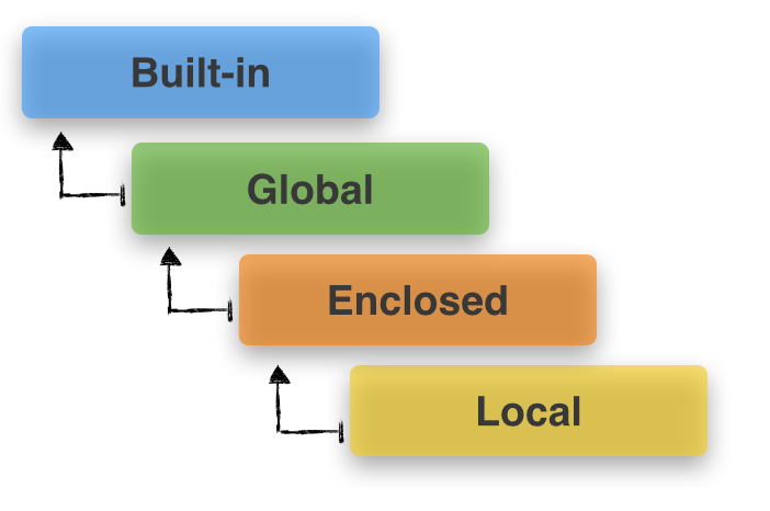
Local:
- Defined in the local scope of functions
def sales_tax(amount):
    rate = 0.0625 # Local variable
    tax_total = amount * rate # rate can be seen here
    total = tax_total + amount
    print(total)

# Call function and pass parameter
sales_tax(200)  # Rate cannot be seen here
Enclosing-Function Global
- Refers to variables defined within local scope of functions wrapping other functions
def program():
    amount = 200 # Enclosing-Function Global variable
    def sales_tax():
        rate = 0.0625
        tax_total = amount * rate # Amount can be seen here
        total = tax_total + amount
        print(total)
    sales_tax() # Amount could be seen here

# Amount could not be seen here
program()
Global/Module
- Variables defined at the top level of files and modules
amount = 200 #Global variable, can be seen everywhere below.

def sales_tax():
    rate = 0.0625
    tax_total = amount * rate
    total = tax_total + amount
    print(total)

# Did not pass parameters
sales_tax()
Built-In
- Loaded into scope when interpreter starts up. (Ex: hash(), min(), dict(), print(), etc)
Modifying Global Variables Within a Different Scope
- We can use the global keyword to grant access to global variables within a different scope, allowing for modification.
Example:
a = 1

# Uses global because there is no local 'a'
def f():
    print('Inside f() : ', a)

# Uses local variable a
def g():
    a = 2
    print('Inside g() : ', a)

# Uses global keyword to grant access to global a, allowing modification
def h():
    global a
    a = 3
    print('Inside h() : ',a)

# Global scope
print('global : ', a)
f()
print('global : ', a)
g()
print('global : ', a)
h()
print('global : ', a)
Output:
global :  1
Inside f() :  1
global :  1
Inside g() :  2
global :  1
Inside h() :  3
global :  3
User Functions
Python functions are blocks of reusable code that can be called to accomplish some sort of functionality. Functions are meant to split up the code into functionally organized code that can be reused. In Python, you do not have to return a value.
To define a function use:
def function_name(parameters):
def function_name(parameters):
    x = 0 # What we want to return

    return x # What we return
With return value:
def name_upper(name):
    name = name*2
    return name
print(name_upper('Cao'))
With no return value:
def name_upper(name):
    <code>
    print(name)
Calling a Function
To call a function, you simply call the function name and pass in any needed arguments. If the function returns a variable, it is wise to call the function and direct the return value into a variable.
# Lets print a name
print_name('SrA. Snuffy')
Another example:
def divisible_by(num, amount):
    i = 1.0
    while (num / i >= 1 and amount > 0):
        if num % i == 0:
            print("{} divided by {} equals: {}".format(num, i, num / i))
            amount -= 1
        i += 1
divisible_by(900, 10)
Parameters and Arguments
Parameters
Parameters are defined within the parentheses; they are undefined variables that you want to use within the function. This keeps the global scope clean. We can specify default parameter values as well as specify type. A lot of this can be done within the parentheses... but this can lead to unexpected problems. Before we get to default parameters, let's go over a very important topic.
Copies vs References
Things are different in Python. Objects are never copied during a function call... EVER. Function parameters are names, that's it. We bind these names to the objects we pass. So in a way, it may seem we are copying objects... but we aren't. Nor does it always seem that way. We are dealing with objects through and through, so this changes how things are done.
- As stated above, parameters are just names. When we pass arguments (and all arguments are objects because everything is an object in Python), we are binding these objects to these names.
- As we've learned, objects are mutable or immutable. The same applies here.
- Objects that are immutable may appear like they are being copied. Because really, there is no way for you to modify the originals without utilizing the global keyword or through reassignment. Instead what happens, when you do varname = (reassigning and not the same as varname[] =), you are creating a new name binding within the function's scope. Changes made within this scope will not be present on other existences of said object in other scopes.
- On the other hand, objects that are mutable may appear like they are being referenced, sometimes they may appear like they are being copied. The above statement is still true. But things go a step farther. When using methods or other mutable actions to act on a mutable object, you will modify the object in all scopes. It's still the same object and no new name binding was created. Let's see some examples to break this down further:
Example of Modification
x = [1,2,3,4] # here we create a global list

def test(x):
    x[1] = 20           # here we are modifying the mutable object via indexing
    x.append(50)        # here we are modifying the mutable object via method

test(x)

print(x)

# output: 1,20,3,4,50
Example of Name Binding
x = [1,2,3,4] # here we create a global list

def test(x):
    x = [1,2,3,4,5]
    x.append(200)

test(x)

print(x)

# output: 1,2,3,4
Default Parameters
Common Way (but risky)
def divisible_by(num, amount = 5):
    i = 1.0
    while (num / i >= 1 and amount > 0):
        if num % i == 0:
            print("{} divided by {} equals: {}".format(num, i, num / i))
            amount -= 1
        i += 1
divisible_by(900, 10)
Safe Way
This forces the default arguments to be evaluated each time the function is called. This is especially important with mutable default objects.
# Checks all numbers that can be divided into num... up until amount has been reached or we reach divide by self
def divisible_by(num, amount=None):
    if amount is None:
        amount = 5

    i = 1.0
    while (num / i >= 1 and amount > 0):
        if num % i == 0:
            print("{} divided by {} equals: {}".format(num, i, num / i))
            amount -= 1
        i += 1
divisible_by(900)
Arguments
Arguments are defined variables that you pass on the function call.
Examples of parameters and arguments:
def sales_tax(amount): # function and parameter 'amount'
    rate = 0.0625
    tax_total = amount * rate
    total = tax_total + amount
    print(total)

sales_tax(200) # Function call and argument 200
*args and **kwargs
- *args are used to pass a non-keyworded, variable-length argument list.
- **kwargs is used to pass a keyworded, variable-length argument list.
- A keyword argument is where you provide a name to the variable as you pass it into the function.
- kwargs are placed in dictionaries.
Example:
def my_func1(*args):
    for arg in args:
        print('arg: ', arg)
        print(type(args))
def my_func2(**kwargs):
    for key, value in kwargs.items():
        print(key, value)
my_func1('two', 3, 'four', 5)
my_func2(a = 12, b = 'abc')
Cmdline Arguments
Arguments can also be passed through the command line or terminal.
Old:
Know both versions. The new version works in both Python 2.7 and 3.x
import sys

args = str(sys.argv)
print(sys.argv[0]) # The name of the program is always argv[0]
for i in range(len(sys.argv)):
    print 'args[%d]: %s' % (i, sys.argv[i])

# Input Example: python2 test.py hello world "Hello World"
# What is the output?
New:
import argparse

parser = argparse.ArgumentParser(description='This is a demo')
parser.add_argument('-i','--input',help='Input arg', required=True)
args = parser.parse_args()

print(args.input)

# Input Example: python2 test.py -i test
Reference: Argparse Tutorial
Returning
With functions, you have the choice to return a variable. This is done so that the function becomes it's own local scope... keeping the global scope clean from any interference that the function may cause. If you want to bring a local function variable outside of the local scope... return a variable. With that said, returned values can be reassigned. If you find yourself having to return a ton of variables, either use a sequence or mapping object or split up the functionality into additional functions.
def create_initials(first_name, last_name):
    initials = first_name[0].upper() + last_name[0].upper()
    return initials

initials = create_initials("jack", "black")
print(initials)
Pass by Reference
Pass by Object Reference simply means that objects passed to the functions are referenced. This is technically what Python does by default. Since the objects are referenced, it can be easy to change the contents of that object; especially mutable objects.
#Define the function
def append_one(a):
    a.append(1)

# Declare and set a variable
a = [0]
# Pass that variable by reference to the function append_one()
append_one(a)
print(a)

# Since the function acted on a mutable variable... the contents of the object were changed.
[0, 1]
Practical Example
The following code contains a bit of everything we have learned including some things we have not learned. This is a more robust and error/hack proof version of divisible_by that we looked at above.
"""
Checks a certain range of numbers to see if they can divide into a user specified num
"""
# Program main, runs at start of program
def launch():
    num = raw_input('What number would you like to check?')
    amount = raw_input('How many numbers do you want to check?')

    if isInt(num) == False or isInt(amount) == False:
        print("You must enter an integer")
        launch()
    elif int(amount) < 0 or int(num) < 0:
        print("You must enter a number greater than 0")
        launch()
    else:
        divisible_by(int(num), int(amount))

# Checks num divisable numbers up to amount or itself
def divisible_by(num, amount):
    i = 1.0
    while (num / i >= 1 and amount > 0):
        if num % i == 0:
            print('{} is divsible by {}'.format(int(num), int(i)))
            amount -= 1
        i += 1

# Checks if string represents an int
def isInt(x):
    try:
        int(x) ###
        return True
    except ValueError:
        return False

launch()
Lambda Functions
It's best to start off with some examples:
Example 1:
my_list = range(26)

print(my_list)
print(filter(lambda x: x % 2 == 0, my_list))
Breaking down the first example:
lambda - the keyword to create a lambda
x - the parameter. Multiple parameters ex: lambda x,y,z:
x % 2 == 0: the execution code
my_list: the argument. Multiple args ex: lambda x,y,z: <code>, input1, input2, key

Multiple arg/param lambda:
lambda x,y,z: (x + y) - z, input1, input2, key
Example 2:
g = lambda x,y: x>y
print g(1,2)
print g(2,1)
As you can tell, lambdas appear to be shortened functions; specifically one lined functions. And while this is true to an extent... that is not their purpose.
Lambdas, in short, are anonymous functions. Functions without a name. They are generally passed as arguments to higher-order functions as well as a variety of other uses. Below are some of the features of a Lambda
Lambda Features:
- Lambda forms can take any number of arguments
- Return only one value in the form of an expression
- They cannot contain commands or multiple expressions
- It cannot be a direct call to print because lambda requires an expression
- Lambda functions have their own namespace
Due to the fact that they have their own local namespace... Lambdas cannot access variables other than those in their parameters list and globals.
Example:
def factorial(n):return reduce(lambda x,y:x*y,[1]+range(1,n+1))
Breakdown of a Lambda
#Define a regular function
def reg_function(x):
    return x**2

# Make it one line
def reg_function(x): return x**2

# Turn it into a lambda
new_stuff = lambda x: x**2
Common Lambda Uses
map()
- Map applies a function to all the items in an input_list. That function can be a lambda.
filter()
- Filter creates a list of elements for which a function returns true.
reduce()
- Reduce accepts a function and a sequence and returns a single calculated value.
Examples
Continue to Performance Labs: 4A and 4B
Lab 4A & 4B
Lab 4A: Calculator
Instructions
Create a fully functional calculator using BOTH functions and lambdas. Create a user menu as well as a "screen" where the numbers and operations take place. The calculator needs to have the following functionality:
- Addition
- Subtraction
- Division
- Multiplication
- Power
- At least two math algorithms (One can be your Fibonacci)
Requirments
- Adhere to PEP8
- Functionality requirements above
- Utilize user input and proper validation
- Utilize proper formatting
- Utilize proper and clean statements and loops
Additional
- More than two numbers
- Continuous operations (5 + 5 + 2 - 1 / 2 for example)
- Additional operations
- Additonal math algorithms
- etc
Lab 4B: Lab 3E Part 2
- Return to Lab 3E and follow instructions for Fibonacci recursive function.
List Comprehension
Python supports something called "list comprehension". In short, this allows us to write minimal, easy and readable lists in a way like mathematicans do. Essentially you put everything in a one liner.
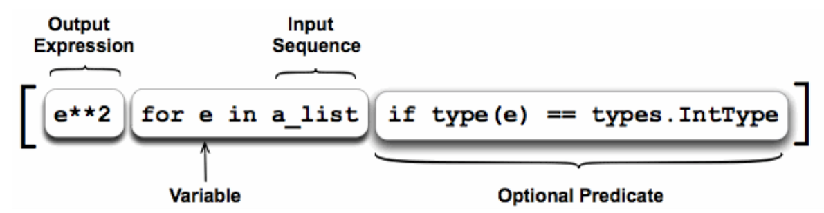
Steps
Taking a look at the example above, let's break it down into something more understandable.
- First, the for e in a_list is examined.
- a_list is just some var list that is visable within our scope
- We are going to iterate through this list...
- While itterating through the list, we are going to check the optional predicate, if type(e) == types.IntType in this case
- So per iteration, we check that condition. If it's true, we execute the output expression...
- As per the name, it's optional. If there is no optional predicate, the output expression simply runs.
- The output expression, e**2 in this case, is ran if the optional predicate exists and is True.
- This happens per iteration of a_list as well.
Normal List
a_list = [1,2,3,4,5]

def square_list(a_list):
    a = []
    for item in a_list:
        a.append(item*item)
    return a

print(square_list(a_list))

# Output
[1, 4, 9, 16, 25]
Normal List with Refactoring
(In this example the a_list global variable was overwritten. This can be avoided by reassigning the results to a new variable.)
a_list = [1,2,3,4,5]

def square_list(a_list):
    for i in range(len(a_list)):
        a_list[i] *= a_list[i]

square_list(a_list)
print(a_list)

# Output
[1, 4, 9, 16, 25]
List Comprehension Without Conditional
a_list = [1,2,3,4,5]

def square_list(a_list):
    return [x*x for x in a_list]

print(square_list(a_list))

#Output
[1, 4, 9, 16, 25]
List Comprehension With Conditional
a_list = [1,2,3,4,5]

def square_list(a_list):
    return [x*x for x in a_list if x % 2 == 0]

print(square_list(a_list))

# Output
[4, 16]
Set Comprehension With Conditional
Instead of using brackets [ ] as you would for lists you use curly braces { } like you would for a set.
a_list = [1,2,3,4,5]

def square_list(a_list):
    return {x*x for x in a_list if x % 2 == 0}

print(square_list(a_list))

# Output
set([16, 4])
If you are looking to get rid of duplicates within a list then using Set Comprehension is good for this.
# This list has duplicates
b_list = [1,2,2,3,4,4,5]

def square_list(b_list):
    return [x*x for x in b_list]

squared_list = square_list(b_list))
print(squared_list)
# We can convert this list to a set by using the set() method
set(squared_list)


# Why do the extra steps when we can just use set comprehension
def square_set(b_list)
    return {x*x for x in b_list}

squared_set = square_set(b_list))
print(squared_set)
Dictionary Comprehension
Dictionary comprehension is a great way to take one dictionary and transform, or conditionally include items into a new dictionary. Just remember not to make these too complex. Their main purpose is to make your code more readable.
my_dict = {'a': 1, 'b': 2, 'c': 3, 'd': 4, }

squared_dict = {k:v*v for (k,v) in my_dict.items()}
print(squared_dict)
Recursion
Recursion is a function that calls itself. In other words a function will continue to call itself until a certain condition is met. Any problem that can be solved by recursion can be solved by using a loop. We mentioned before that it is almost always preferential to use a loop due to overhead. However, you may want to use recursion when you have a problem that needs to be broken into smaller similar problems and solve them first.
Base case and recursive case
Base Case
If the problem can be solved now, then the function solves it and returns
Recursive Case
If the problem cannot be solved now, then the function reduces it to smaller similar problems and calls itself to solve the smaller problem.
Recursion to find factorial of a number
The best way to understand is to dive in. Lets take a look at solving for n!. As a quick reminder n! is defined as:
    n! = n x (n-1) x (n-2) x (n-3) x...x 3 x 2 x 1
    4! = 4 x 3 x 2 x 1 = 24

Base case:
    If n = 0 then   n! = 1
or  If n = 0 then   factorial(n) = 1

Recursive case:
    If n > 0 then   n! = 1 x 2 x 3 x ... n
or  If n > 0 then   factorial(n) = n x factorial(n-1)
Now lets translate to Python:
def recursive_factorial(n):
    #base case
    if n == 0:
        return 1
    #recursive case
    else:
        return n * recursive_factorial(n-1)
Be sure that every time you write a recursive function that you can control the number of times it will be executed.
# Endless recursion
def forever_recursion():
    annoying_message()

def annoying_message():
    print('Nudge Nudge, Wink Wink, Say No More Say No More')
    message()

Recursion for the Fibonacci Series
A very common way to present recursion is by writing a program to calculate Fibonacci numbers. After the second number, every number in the series is the sum of the two previous numbers. The sequence is the following: 0,1,1,2,3,5,8,13,21,34,55,89,144,233,...
A recursive function can have multiple base cases. Both of them return a value without making a recursive call.

Base case:
    If n = 0 then   fibonacci(n) = 0
    If n = 1 then   fibonacci(n) = 1

Recursive case:
    If n > 1 then   fibonacci(n) = fibonacci(n-1) + fibonacci(n-2)
Now lets translate to Python:
def fibonacci(n):
    if n == 0:
        return 0
    elif n == 1:
        return 1
    else:
        return fibonacci(n-1) + fibonacci(n-2)
Closures, Iterators & Generators
Closures
A Closure is a function object that remembers values in enclosing scopes regardless of whether those scopes are still present in memory. If you have written a function that returned another function, you probably have used closures without even knowing.
Example:
def generate_power_func(n):
    def nth_powah(x):
        return x**n
    return nth_powah


x = generate_power_func(10)
print(x)
# What happens? How is this possible?
def generate_power_func(n):
    def nth_powah(x):
        return x**n
    return nth_powah


x = generate_power_func(10)
print(x)

y = x(4)
print(y)

# What happens now?
Why Use Closures?
- Closures can avoid the use of global values and provide some form of data hiding.
- They provide a layer of simplicity
Why to Avoid Closures?
- They are harder to debug
- They may not always be cleaner
- They can get complex quickly
Iterators
An iterator is just an object with a state that remembers where it is during iteration, something that can be looped upon. We've gone over some Iterable objects like for loops, strings, lists, dictionaries, etc. Now we will learn how to make our own iterator using iter object.
Why use Iterators?
Building your own iterator means that you can save memory space. If you have a very large data set you can use iterators for lazy evaluation.
Example of iter function:
>>> x = iter([1, 2, 3, 4, 5, 6])
>>> print(x)
<listiterator object at 0x02B2AB30>
x.next()
1
x.next()
2
x.next()
3
x.next()
4
x.next()
5
x.next()
6
x.next()
Traceback (most recent call last):
  File "<stdin>", line 1, in <module>
StopIteration
The one we will be using the most is the range() function. Below is an iterator, implemented as a class that works like range. This is your first major look at classes... don't freak out! Let's break this down.
class yrange:
    def __init__(self, n):
        self.i = 0
        self.n = n

    def __iter__(self):
        return self

    def next(self):
        if self.i < self.n:
            i = self.i
            self.i += 1
            return i
        else:
            raise StopIteration()

# using y range
yrange(3)
y.next()
0
y.next()
1
y.next()
2
y.next()
Traceback (most recent call last):
  File "<stdin>", line 1, in <module>
  File "<stdin>", line 14, in next
StopIteration
As we learned in the Data Types lecture... range() loads one at a time. The yrange() class here does the same thing. There are lists, tuples, etc... loaded up. Instead, we deal with two variables: i and n.
Generators
Generators are also iterators (iterators are not always generators though). Generators simplify the creation of iterators. A generator is simply a function that produces a sequence of values to iterate through rather than a single value.
Before we go over the example lets discuss yield. Yield is similar to return however yield produces a sequence of values. If there is a yield in the body of the function then it is a generator.
def yrange(n):
    i = 0
    while i < n:
        yield i
        i += 1
my_gen = yrange(10)
print(my_gen)
for i in my_gen:
    print(i)

# output
<generator object yrange at 0x007F3328>
0
1
2
3
4
5
6
7
8
9
Taking a look at the code above... we created a sequence object and iterated over it using a for loop.
Note: When functions return all state is lost, a yield preserves local state and returns a generator object.
Object Oriented Programming
Introduction:
This lesson you will walk through Object-oriented Programming, or OOP for short, which bundles attributes and methods into individual objects. Here you will learn how to create and use objects using Object-Oriented Programming principals.
Topics Covered:
- Modules
- Packages
- User Classes Pt. 1
- User Classes Pt.2
- Composition vs Inheritance
- Exception Handling
- Object Oriented Programming Principles
- Object Oriented Programming Terminology Review
To access the Object Oriented Programming slides please click here
Lesson Objectives:
-
LO 1 Understand how to import modules and module components in Python. (Proficiency Level: C)
- MSB 1.1 Employ the Python standard library to solve a problem. (Proficiency Level: C)
-
LO 2 Describe how to utilize PIP to install a Python package. (Proficiency Level: B)
-
LO 3 Comprehend Python objects
- MSB 3.1 Comprehend Python classes
- MSB 3.2 Differentiate between Python objects and classes
-
LO 4 Explain the Python keyword super
-
LO 5 Explain Python object initialization
-
LO 6 Explain Python object attributes
-
LO 7 Describe polymorphism in Python
-
LO 8 Describe inheritance in Python
-
LO 9 Describe getter and setter functions in Python
-
LO 10 Understand how to implement input validation in Python.
-
LO 11 Understand how to implement exception handling in Python.
-
LO 12 Describe the terms and fundamentals associated with object-orientated programming using Python. (Proficiency Level: C)
- MSB 12.1 Describe the advantages of object-orientated programming in Python. (Proficiency Level: A)
-
LO 13 Discuss Common Principles of object-oriented programming.
-
LO 14 Discuss Code Styling Considerations of object-orientated programming.
Performance Objectives (Proficiency Level: 3c)
-
Conditions: Given access to (references, tools, etc.):
- Access to specified remote virtual environment
- Student Guide and Lab Guide
- Student Notes
-
Performance/Behavior Tasks:
- Create, reuse and import modules in Python.
- Utilize modules in the Python standard library.
- Install and utilize a Python package via PIP.
- Write a class in Python
- Instantiate a Python object
- Write a class constructor
- Write object-oriented programs
- Implement object inheritance.
- Expand class functionality using getter and setter functions.
- Use class methods to modify instantiated class objects.
- Write a program to demonstrate input validation in Python.
- Write a program to demonstrate exception handling in Python.
-
Standard(s)
- Criteria: Demonstration: Correctable to 100% in class
- Evaluation: Students will have 4 hours to complete the timed evaluation consisting of both cognitive and performance components.
- Minimum passing score is 80%
Modules
Modules are reusable code that can be imported into other scripts or programs. Modules are single files in either .py, .pyc or .pyo format. When a module is imported, code that is not wrapped in a function is executed and the functions themselves are added to the namespace... allowing them to be called upon.
Module Structure
#/usr/lib/python/site-packages/triangle.py

divisor_count_to_find = 500

def triangle_number(n):
    return n*(n+1)/2

def divisors(tn):
    counter = 0
    n_sqrt = int(pow(tn, 0.5))
    for i in range(1, n_sqrt + 1):
        if tn%i == 0:
            counter += 2
    if n_sqrt * n_sqrt == tn:
        counter -= 1
    return counter

def start():
    start_number = 1
    div_numbers = 0
    while (div_numbers < divisor_count_to_find):
        tn = triangle_number(start_number)
        div_numbers = divisors(tn)
        start_number += 1
    print(div_numbers)
    print(tn)

if __name__ == '__main__':
    start()
Reference: if __name__ == '__main__':
In other words, a module is a file containing Python definitions and statements. The file name is the module name with the suffix .py appended (every .py file is a module). Within a module, the module’s name (as a string) is available as the value of the global variable __name__.
Using Modules
- First, we import the module. We will learn more coming up.
- After the module is imported we can begin utilizing the module's objects.
- When a module is imported normally, the module will be on it's own namespace.
- Thus we need to use dot notation to access the modules objects
import triangle
triangle.start()
triangle.triangle_number(10)
triangle.divisors(10)
triangle.divisor_count_to_find = 100

triangle.start()
# 576 76576500.0 112 73920.0
Importing Modules
There are many ways to import modules. The most common way is to import the module simply using the import keyword alone. These modules are imported from the same dir as your program. This method prevents collisions by putting the modules objects into it's own namespace.
# Most common, clean way to do it. Prevents collisions.
import triangle
triangle.method # Call method
By default, you cannot import modules from other dirs. You must place your modules in the same dir as your program unless you use sys.path to modify your Python path at runtime. In short, your Python path is where Python searches by default for modules... aside from your current dir.
To add a location to your Python path and runtime:
import sys
sys.path.insert(0, '/path/to/application/app/folder')

import file
There are other methods as well. We can give our modules aliases
# Same as above except we gave triangle an alias
import triangle as tri
tri.method
We can also import specific modules without throwing them into a namespace.
from triangle import divisor_count_to_find, triangle_number

print divisor_count_to_find # output 500
triangle_number(5)
We can take the previous example a step further and implement aliases. This will allow us to change the names up to prevent collisons.
from triangle import divisor_count_to_find as dcf, triangle_number as tn

print dcf # output 500
tn(5)
Lastly, we can also import an entire module without a namespace. The * tells Python to import all modules without a namespace. This is a dangerous method and should only be used if you are sure there will not be collisions.
from triangle import *
Reference: Modules
Packages
Packages are a way to structure Python's module namespace. Essentially a package is just a collection of modules. A module named __init__.py is required to treat the directory as a package; allowing the package to be imported the same way a module can be imported. This file can contain initialization code... but it's often best to leave it blank.
Package Structure
/                       # Top directory
    math_stuff/         # Package
        __init__.py     # special file
        fib.py          # fib module
        triangle.py     # triangle module
        Calculator.py   # calculator class module
    more_math_stuff/    # additional package
        __init__.py
        other_modules.py
How to Import From a Package
So let's take the package below and walk through an import.
/                       # Top directory
    math_stuff/         # Package
        __init__.py     # special file
        fib.py          # fib module
        triangle.py     # triangle module
        Calculator.py   # calculator class module
    more_math_stuff/    # additional package
        __init__.py
        other_modules.py # import and run this file (module)
There are two ways we can go about this:
import more_math_stuff.other_modules

more_math_stuff.other_modules.do_something()
OR
from more_math_stuff import other_modules as om

om.do_something()
Notice the calls to the module. They do behave differently. You can also import the entire package as well.
Useful Commands
- dir()
- Returns list of names in current local scope or with argument, attempts to return a list of valid attributes for object
- help()
- Invokes built-in help system
# dir
>>> print dir()
['__builtins__', '__doc__', '__name__', '__package__']
>>> import(struct)
>>> print dir()
['__builtins__', '__doc__', '__name__', '__package__', 'struct']
>>> print dir(struct)
['Struct', '__builtins__', '__doc__', '__file__', '__name__', '__package__', '_clearcache', 'calcsize', 'error', 'pack', 'pack_into', 'unpack', 'unpack_from']

# help
print help(struct)
# Try it
print help()
# Try it
Continue to Lab 5A
Lab 5A
Instructions
Using your calculator you created from Lab4A, split up the functionality into modules and utilize packaging. Some things you could split up:
- The user menu into it's own module on a higher level package
- Operations into one module, lower level
- Algorithms into one module, lower level
- etc
Requirements
- All requirements from Lab4A
- Utilize clean and proper dir and module names
User Classes Pt1
Classes are used to create objects that bundle data and functionality together. With this, classes are highly reusable, cleaner and more efficient. In other languages, some entites are objects and some are not. In Python, everything is an object. Classes and built-in types were at one point different. But that has all since been merged and both are now objects of type type. (more to come on this later) Here are some considerations:
Keywords
Reserved words of the language, and cannot be used as ordinary identifiers. Do not use any of these for any naming. They must be spelled exactly as written here:
and       del       from      not       while
as        elif      global    or        with
assert    else      if        pass      yield
break     except    import    print
class     exec      in        raise
continue  finally   is        return
def       for       lambda    try
To verify that a string is a keyword you can use keyword.iskeyword; to get the list of reserved keywords you can use keyword.kwlist:
>>> import keyword
>>> keyword.iskeyword('break')
True
>>> keyword.kwlist
['False', 'None', 'True', 'and', 'as', 'assert', 'break', 'class', 'continue', 'def',
 'del', 'elif', 'else', 'except', 'finally', 'for', 'from', 'global', 'if', 'import',
 'in', 'is', 'lambda', 'nonlocal', 'not', 'or', 'pass', 'raise', 'return', 'try',
 'while', 'with', 'yield']
Creating a Class
Let's take a quick look at an example of a class, using the famous Person example. This example is very basic and will be expanded upon as we go.
# This is the class
class Person:
    """Stage 1 of Person Class

    We will expand on this."""

    firstName = "James"
    lastName = "Bond"
    birthday = "08/21/1800"
    age = "200"
    email = "[email protected]"

    def f(self):
        return "This is the Person class"

# This is the instantiation of class Person as object x
x = Person()

# This is using object x
print x.f()
print "This person's name is: {} {}".format(x.firstName, x.lastName)

# We can also do this...
print Person.firstName
Let's take a look at what we have above.
- To create a class, we use the class keyword followed by the class name.
- Notice, the name starts with a capital letter. This is following PEP8 standards.
- Inside the class, we created a multi-line docstring. Generally at least a single line docstring is needed.
- Below that, we have some Class Variables: firstName, lastName, birthday, age and email. These are varibales shared between all instances of a class.
- We also have Instane Variables which belong only to that instance. These are generally defined within Methods.
- Below the class variables, we have a method f. This is the same thing as a member function we are used to in C++.
- After the creation of the class itself, concepts start to blur between Python and C++.
- Notice we call Person() and assign it's value to x. This is called class instantiation. This is a concept we should already be used to thanks to C++.
- x now holds our object, from here we can access all public class variables and methods. In our case, everything is public.
- We do just that on the next line, printing x.f(). Just like C++, we use dot-notation to access class variables and methods.
- x.f() calls the f() method of class Person, object x.
- We then access class variables firstName and lastName on the next line and print them out.
- Finally, the last line. Notice we don't access object x, instead we access the class directly. Remember, even class creation and types are objects. So what does this mean?
- We have something called attribute references in Python.
- This allows us to access a classes attributes... meaning, we can modify things on the class level, even after instances are created. Changes are displayed across the board on all instances only if the instance's variable wasn't modified first. If it was, that variable no longer shares a connection with the class and becomes a sole instance variable. Let's take a look at an example in the interactive terminal.
>>> class someClass:
...     x = 100
...
>>> someClass.x
100
>>> someInstance = someClass()
>>> someInstance.x
100
>>> someClass.x = 400
>>> someInstance.x
400
>>> someInstance.x = 1000
>>> someInstance.x
1000
>>> someClass.x = 0
>>> someInstance.x
1000
So as we have seen above, despite it being a basic example of a class, it already seems very useful. But classes get much better in Python. Let's cover some other class concepts.
__init__()
It is possible to create objects with instances customized to a specific state. Just like C++, we have the ability to construct objects. But we also have the ability to customize objects. These two things are different. __init__() is not a constructor. Instead, this comes after the constructor and allows us to customize our object. __new__() on the otherhand is the constructor. We will not be going over the use of __new__().
self
Before we can continue on __init__(), we need to understand the word self. The self in python represents or points the instance which it was called. Remember the difference between instance variables and class variables? One is tied to only the specific instance and the other is tied to all instances. Well, we went over how to create and modify class variables. We also went over how to convert one to a instance variable. But how do we create instance variables with the intention to do so? That's where self comes in. It's best if we take a look at another Python Interpetor example.
>>> class someClass:
...     ex1 = 0
...     ex2 = 0
...
...     def f(self, val):
...             ex1 = val
...             self.ex2 = val
...
>>> # the class has been created. We also created a method.
... # the method attempts to change ex1 and self.ex2 to val
...
>>> someInstance = someClass()
>>> someInstance.ex1
0
>>> someInstance.ex2
0
>>> someInstance.f(100)
>>> someInstance.ex1
0
>>> someInstance.ex2
100
- Notice how we had this method
f().f()has two arguments,selfandval.selfas we said above, represents the specific instance for which it was called. When the method is called, self is automatically populated by Python. So there is no need for us to pass a self argument.valwill be our argument which changesex1andex2- Now, let's assume we got rid of this class and converted the class variables to normal global variables and the
f()method to a regular function.- If we wanted to modify a global variable within a function, we would have to define
global ex1before acting onex1 - This concept is kinda the same for
selfwithin classes... except the scope stops at that of the instance rather than accessing the global.
- If we wanted to modify a global variable within a function, we would have to define
- Once we created our instance and called the
f()method... we observed it only changedex2. This is becauseselfaccessed the instance and grabbed it's instance variable rather than creating a new variable within the function scope.
In short, by using self... we are telling Python that we want to modify the classes instance variables rather than create/modify variables local to something else such as a method.
Utilizing __init__()
Now that we have a general understanding of self, let's create a __init__() method.
We can do something as simple as:
class X:

    def __init__(self):
        self.i = "yay"

# Invalid
print X.i  # We will get an error, i is not a class variable

# Valid
a = X()
print a.i  # Output will be 'yay'
This prevents us from being able to change data across all classes. But we have even more flexibility than that in Python, we can also pass additional arguments to __init__() via on object instantiation.
def __init__(self, firstName, lastName):
    self.firstName = firstName
    self.lastName = lastName


# Once we go to create the object
x = Person("James", "Bond")
Now that we have learned how to utilize __init__()... let's update our example.
# This is the class
class Person:
    """Stage 2 of Person Class

    We will expand on this."""

    def __init__(self, firstName, lastName, birthday, age, email):
        self.firstName = firstName
        self.lastName = lastName
        self.birthday = birthday
        self.age = age
        self.email = email

    def printDetails(self):
        print "First Name: {}".format(self.firstName)
        print "First Name: {}".format(self.lastName)
        print "First Name: {}".format(self.birthday)
        print "First Name: {}".format(self.age)
        print "First Name: {}".format(self.email)

# This is the instantiation of class Person as object x
x = Person("James", "Bond", "08/21/1800", 200, "[email protected]")
x.printDetails()
Continue to Performance Lab: 5B
Lab5B
Instructions
Create a very simple super hero class. Some attributes you will need:
- Hero Name
- Real Name
- Power(s)
- Colors
- etc
Requirements
- Adhere to PEP8 and utilize proper and efficient code
- Utilize an
__init__() - Ensure variables are correct type (class vs instance variables)
- Utilize methods:
- Start to format your class using getters and setters
- Create an instance of your class. Populate it with data utilzing an init and/or getters and setters
Additional:
- Begin using encapsulation techniques
User Classes Pt2
Encapsulation in Python
In C++ and other languages, encapsulation is harped on pretty hard and the languages give you features that really allow for such a mechanism. In Python? Not so much. Well, not to the level of which we are used to.
Public
All member variables and methods are public by default in Python. Just do as you do if you want public.
"Protected"
A protected member (in C++ and Java) is accessible only from within the class and it’s subclasses. In C++, we can create idiot-proof ways to really protect things members. In Python? Well, it's more of a suggestion. By prefixing the name of your member with a single underscore, you’re telling others “don’t touch this, unless you’re a subclass”. And by others... we mean other programmers. Yes, you can still access the members outside of the class.
class Example:
    def __init__(self, name):
        self.name = name
        self._number = None # "protected" variable
        self._displayName()

    def _displayName(self):
        print "Hello, {}".format(self.name)

    def setNumber(self, num):
        self._number = num

    def getNumber(self):
        return self._number

print "====Proper Things====\n"
a = Example("Will")
a.setNumber(21012345678)
print a.name
print a.getNumber()


print "====Does it really work?====\n"
print a._number
a._displayName()
"Private"
Same thing really applies here. By declaring your data member private you mean, that nobody should be able to access it from outside the class. Python supports a technique called name mangling. This feature turns every member name prefixed with at least two underscores and suffixed with at most one underscore into _<className><memberName>
class Example:
    def __init__(self, name):
        self.name = name
        self.__number = None # "private" variable
        self.__displayName()

    # private method
    def __displayName(self):
        print "Hello, {}".format(self.name)

    def setNumber(self, num):
        self.__number = num

    def getNumber(self):
        return self.__number

print "====Proper Things====\n"
a = Example("Will")
a.setNumber(21012345678)
print a.name
print a.getNumber()

print "====How to get around it====\n"
print a._Example__number    # This works, though it is much more confusing and even throws errors
Python Specific Breakdown
__init__ (Constructor)
__del__ (Deconstructor)
- It's best to name the Python file after the class name/vise-versa.
class ClassName(object):-- to define class- Name classes using CapWords convention (camel-case)
- Variables defined under classes are shared though all instances
- Variables defined in methods using
selfare only for a single instance - When creating methods, the first parameter must be self. (similar to "this" in other languages)
- A "private" member can be created by prepending a double underscore (only prepend) to the name. It will not be visable outside of the class. __example
- Inheritance, multiple inheritance and polymorphism are all supported
- var.attrib = value is the common way to interact(dot notation)
- getattr, hasattr, setattr, delattr exist for manipulating attributes as well
- built in:
__dict__, __doc__, __name__, __module__, __bases__
- Overloadable:
__init__, __del__, __repr__, __str__, __cmp__
- dir(), type(), isinstance() are built in functions
Creating an Instance in a Different File
from MyClass import MyClass

x = MyClass(name = "Iron Man")
print x.getName()
Composition vs Inheritance
- Best advice is composition over inheritance, but use inheritance when needed.
- Inheritance can complete things (especially multiple inheritance) and make larger projects confusing
- Namespace collisions are a major problem in inheritance
- Time must be given to design to effectively use inheritance, which could be time used used to stand up composition quicker.
Inheritance Example
Parent Class
class Person(object):
    def __init__(self, name):
        self.__name = name
        self.__age = None
        try:
            firstBlank = self.__name.rindex(' ')
            self.__lastName = self.__name[firstBlank+1:]
        except:
            self.__lastName = None

    def getLastName(self):
        return self.__lastName

    def setAge(self, age):
        self.__age = age

    def getAge(self):
        if age == None:
            return "N/A"
        else:
            return self.__age
Child Class
from Person import Person

class USResident(Person):
    """A person who resides in the US"""

    def __init__(self, name, status):
        Person.__init__(self, name)

        if status.lower() != 'citizen' and /
        status.lower() != 'legal_resident' and /
        status.lower() != 'illegal_resident':
            raise ValueError()
        else:
            self.__status = status

    def getStatus(self):
        """
        Returns the status
        """
        return self.__status
Example Call
from USResident import USResident

resident = USResident("Joe Smo", "citizen")
resident.setAge(23)

print "{} is a {} and is {} years of age.".format(resident.getLastName(), resident.getStatus(), resident.getAge())
Composition Example
class Engine:

    def __init__(self, size, amount):
        self.size = size
        self.amount = amount

    def calculatePower(self):
        return self.size * self.amount

class Payload:

    def __init__(self, name, typeOf, weight):
        self.name = name
        self.typeOf = typeOf
        self.weight = weight

    def neededPower(self):
        return self.weight * .25

class AtlasRocket:

    def __init__(self, size, amount, name, typeOf, weight):
        self.Engine = Engine(size, amount)
        self.Payload = Payload(name, typeOf, weight)

    def missionCapable(self):
        power = self.Engine.calculatePower()
        neededPower = self.Payload.neededPower()

        if power > neededPower:
            return True
        else:
            return False

    def printMissionStats(self):
        print "Avaliable power: {}".format(self.Engine.calculatePower())
        print "Needed Power: {}".format(self.Payload.neededPower())


atlasV = AtlasRocket(200, 4, "DSCS", "COMM", 2000)

if atlasV.missionCapable() == True:
    print "Mission is a go"
    atlasV.printMissionStats()
else:
    print "Mission is not a go"
    atlasV.printMissionStats()
Function vs Method
A function is a piece of code that is called by name. It can be passed data to operate on (i.e., the parameters) and can optionally return data (the return value). All data that is passed to a function is explicitly passed.
def sum(num1, num2):
    return num1 + num2
A method is a piece of code that is called by name that is associated with an object. In most respects it is identical to a function except for two key differences.
- It is implicitly passed for the object for which it was called.
- It is able to operate on data that is contained within the class (remembering that an object is an instance of a class - the class is the definition, the object is an instance of that data).
class Dog:
    def my_method(self):
        print "I am a Dog"

dog = Dog()
dog.my_method()  # Prints "I am a Dog"
More Material
Continue to Performance Lab 5C
Lab5C

Instructions
Update your hero class lab with the following additions:
- Create a generic Person class
- Create a Hero class that inherits from Person
- Refactor code where needed
- Utilize proper Encapsulation
- Include user input
- Use getters and setters
Requirments
- Adhere to PEP8 and utilize proper and efficient code
- Input validation
- Utilize a
__init__() - Ensure variables are correct type (class vs instance variables)
- Utilize methods for getters and setters
- Create a few instances of your class. Populate it with data utilizing an init and/or getters and setters
- Split your classes into separate files and import them properly
Additional:
- Expand this program into a game or larger program. Some possible ideas:
- Hero vs Villan
- Battle Royal
- Guess that Hero
- etc
Exceptions
Python exceptions allow you to attempt code that may result in an error and execute additional functionality on said error.
- Try/except/finally/else
- Try statement begins an exception handling block
- Raise
- Triggers exceptions
- Except
- Handles the exception
- Multiple Exceptions
- Handles multiple exceptions
Example
try:
    <statements>
except: <name>:
    <statements>
except: <name> as <data>:
    <statements>
else:
    <statements>

try:
    <statements>
finally:
    <statements>
Example 2:
"""
Checks a certain range of numbers to see if they can divide into a user specified num
"""
# Program main, runs at start of program
def launch():
    num = input('What number would you like to check?')
    amount = input('How many numbers do you want to check?')

    if isInt(num) == False or isInt(amount) == False:
        print("You must enter an integer")
        launch()
    elif int(amount) < 0 or int(num) < 0:
        print("You must enter a number greater than 0")
        launch()
    else:
        divisible_by(int(num), int(amount))

# Checks num divisible numbers up to amount or itself
def divisible_by(num, amount):
    i = 1.0
    while (num / i >= 1 and amount > 0):
        if num % i == 0:
            print('{} is divisible by {}'.format(int(num), int(i)))
            amount -= 1
        i += 1

# EXCEPTION HANDLING
def isInt(x):
    try:
        int(x) ###
        return True
    except ValueError:
        return False

launch()
class CustomError(Exception):
    def _init_(self, msg):
        self.msg = msg

    def _str_(self):
        return "your error is {}".format(self.msg)

    def doStuff(danger):
        if danger == True:
            raise CustomError("Whoa don't do that!")
            print("Success") #What happens here?

try:
    doStuff(True)

except CustomError as stuff:
    print(stuff)
OOP Principles
Object Oriented: Programming typified by a data-centered (as opposed to a function-centered) approach to program design.
The Zen of Python
Beautiful is better than ugly.
Explicit is better than implicit.
Simple is better than complex.
Complex is better than complicated.
Flat is better than nested.
Sparse is better than dense.
Readability counts.
Special cases aren't special enough to break the rules.
Although practicality beats purity.
Errors should never pass silently.
Unless explicitly silenced.
In the face of ambiguity, refuse the temptation to guess.
There should be one-- and preferably only one --obvious way to do it.
Although that way may not be obvious at first unless you're Dutch.
Now is better than never.
Although never is often better than
right
now.
If the implementation is hard to explain, it's a bad idea.
If the implementation is easy to explain, it may be a good idea.
Namespaces are one honking great idea -- let's do more of those!
—Tim Peters
Capturing the essential internal state and methods that cause state change is the first step in good class design. We can summarize some helpful design principles using the acronym S.O.L.I.D.:
-
Single Responsibility Principle
A class should have one clearly defined responsibility.
-
Open/Closed Principle
A class should be open to extension-generally via inheritance, but closed to modification. We should design our classes so that we don't need to tweak the code to add or change features.
-
Liskov Substitution Principle
We need to design inheritance so that a subclass can be used in place of the superclass.
-
Interface Segregation Principle
When writing a problem statement, we want to be sure that collaborating classes have as few dependencies as possible. In many cases, this principle will lead us to decompose large problems into many small class definitions.
-
Dependency Inversion Principle
It's less than ideal for a class to depend directly on other classes. It's better if a class depends on an abstraction, and a concrete implementation class is substituted for the abstract class.
The goal is to create classes that have the proper behavior and also adhere to the design principles.
Function Style {#ch45lev1sec2}
All the other rules I’ve taught you about how to make a function nice apply here, but add these things:
• For various reasons, programmers call functions that are part of classes methods. It’s mostly marketing but just be warned that every time you say “function” they’ll annoyingly correct you and say “method.” If they get too annoying, just ask them to demonstrate the mathematical basis that determines how a “method” is different from a “function,” and they’ll shut up.
• When you work with classes, much of your time is spent talking about making the class “do things.” Instead of naming your functions after what the function does, instead name it as if it’s a command you are giving to the class. For example, pop essentially says, “Hey list, pop this off.” It isn’t called remove_from_end_of_list because, even though that’s what it does, that’s not a command to a list.
• Keep your functions small and simple. For some reason, when people start learning about classes, they forget this.
Class Style {#ch45lev1sec3}
• Your class should use “camel case” like SuperGoldFactory rather than super_gold_factory.
• Try not to do too much in your __init__ functions. It makes them harder to use.
• Your other functions should use “underscore format” so write my_awesome_hair and not myawesomehair or MyAwesomeHair.
• Be consistent in how you organize your function arguments. If your class has to deal with users, dogs, and cats, keep that order throughout unless it really doesn’t make sense. If you have one function that takes (dog, cat, user) and the other takes (user, cat, dog), it’ll be hard to use.
• Try not to use variables that come from the module or globals. They should be fairly self-contained.
• A foolish consistency is the hobgoblin of little minds. Consistency is good, but foolishly following some idiotic mantra because everyone else does is bad style. Think for yourself.
• Always, always have class Name(object) format or else you will be in big trouble.
Code Style {#ch45lev1sec4}
• Give your code vertical space so people can read it. You will find some very bad programmers who are able to write reasonable code but who do not add any spaces. This is bad style in any language because the human eye and brain use space and vertical alignment to scan and separate visual elements. Not having space is the same as giving your code an awesome camouflage paint job.
• If you can’t read it out loud, it’s probably hard to read. If you are having a problem making something easy to use, try reading it out loud. Not only does this force you to slow down and really read it, but it also helps you find difficult passages and things to change for readability.
• Try to do what other people are doing in Python until you find your own style.
• Once you find your own style, do not be a jerk about it. Working with other people’s code is part of being a programmer, and other people have really bad taste. Trust me, you will probably have really bad taste too and not even realize it.
• If you find someone who writes code in a style you like, try writing something that mimics that style.
Good Comments {#ch45lev1sec5}
• There are programmers who will tell you that your code should be readable enough that you do not need comments. They’ll then tell you in their most official sounding voice, “Ergo one should never write comments. QED.” Those programmers are either consultants who get paid more if other people can’t use their code or incompetents who tend to never work with other people. Ignore them and write comments.
• When you write comments, describe why you are doing what you are doing. The code already says how, but why you did things the way you did is more important.
• When you write doc comments for your functions, make the comments documentation for someone who will have to use your code. You do not have to go crazy, but a nice little sentence about what someone can do with that function helps a lot.
• Finally, while comments are good, too many are bad, and you have to maintain them. Keep your comments relatively short and to the point, and if you change a function, review the comment to make sure it’s still correct.
Reference: PEP8 Style Guide
OOP Terminology Review
Attribute
- Values associated with an individual object. Attributes are accessed using the 'dot syntax':
a.x means fetch the x attribute from the 'a' object.
Argument
- A value passed to a function (or method) when calling the function. There are two types of arguments:
- keyword argument: an argument preceded by an identifier (e.g.
name=) in a function call or passed as a value in a dictionary preceded by**. For example,3and5are both keyword arguments in the following calls tocomplex():
complex(real=3, imag=5)
complex(**{'real': 3, 'imag': 5})
- positional argument: an argument that is not a keyword argument. Positional arguments can appear at the beginning of an argument list and/or be passed as elements of an iterable preceded by
*. For example,3and5are both positional arguments in the following calls:
complex(3, 5)
complex(*(3, 5))
Class
- A template for creating user-defined objects. Class definitions normally contain method definitions that operate on instances of the class.
- Classes provide a means of bundling data and functionality together. Creating a new class creates a new type of object, allowing new instances of that type to be made. Each class instance can have attributes attached to it for maintaining its state. Class instances can also have methods (defined by its class) for modifying its state.
Class Variable
-
Variables defined within the class definition that belong to the class. These variables are shared to all instances of the class.
class TestClass:
    i = 10

print TestClass.i
Constructors
- Fuctions that are automatically called when you create a new instance of a class.
Conditional Statement
- Statement that contains an "if" or "if/else".
Deconstructor
- Called when an object gets destroyed. It’s the polar opposite of the constructor, which gets called on creation. These methods are only called on creation and destruction of the object. They are not called manually but completely automatic.
def
- Defines a function or method
Debugging
- The process of finding and removing programming errors.
Function
- A parameterized sequence of statements.
Syntax
def function_name(parameters, named_default_parameter=value):
  # Some code here
Function/Method Overloading
-
Function Overloading is the ability to create multiple functions with the same name. This allows us to pass different parameters. In Python, this is generally not needed. Instead... we can set default and optional parameters.
def someFunc(x, y, z = None):
    if z is None:
        # Set a default for z or don't use it
    else:
        # Set and use all three

someFunc(1,2)
someFunc(1,2,3)
Generator
- A function which returns an iterator. It looks like a normal function except that it contains
yieldstatements for producing a series of values usable in a for-loop or that can be retrieved one at a time with thenext()function.
Immutable
- An object with fixed value. Immutable objects include numbers, strings and tuples.
Inheritance
- A term used in OOP meaning that classes can inherit from other classes. In other words, it's the transfer of characteristics from one class to another class/classes that are derived from it.
Instance
- An individual object of a certain class.
Instance Variable
-
Similar to Class Variables... except they are only accessible to that one instance. These generally start with the 'self' keyword and are contained within methods.
class NameClass:
    def __init__(self, name):
        self.name = name

dis_class =  NameClass('your_name')
print dis_class.name
#OUTPUT:
'dis_name'
Instantiation
- Instantiation is the act of creating an object instance from a class.
Lambda
- A shorthand to create anonymous functions.
Library
- A library is used loosely to describe a collection of the core modules.The term ‘standard library‘ in Python language refers to the collection of exact syntax, token and semantics of the Python language which comes bundled with the core Python distribution.
Method
- Methods are functions that are called using the attribute notation. There are two flavors: built-in methods (such as append() on lists) and class instance methods. A method is similar to a function but is associated with an object.
Module
- The basic unit of code reusability in Python. A block of code imported by some other code.
Namespace
- A mapping from names to objects. The namespace is a place where a variable is stored in a Python program's memory. Namespaces are implemented as a dictionary. There are the local, global and builtins namespaces and the nested namespaces in objects (in methods).
Nested Scope
- The ability to refer to a variable in an enclosing definition. For instance, a function defined inside another function can refer to variables in the outer function.
Object
- Any data with state (attributes or value, etc...) and defined behavior (methods or functions, etc...). An object can be assigned to a variable or passed into a function as a argument. It's a unique data structure that's defined by it's type or class, etc... Everything in Python is an object.
Operator Overloading
- Operator Overloading is the ability to change the meaning of an operator. This is often done by assigning more than one function to a particular operator.
Package
- A directory of Python module(s). (Technically, a package is a Python module with an
__path__attribute.)
Parameter
- A named entity in a function (or method) definition that specifies an argument (or in some cases, arguments) that the function can accept.
Polymorphism
- The ability to leverage the same interface for different underlying forms such as data typesclasses or functions. This permits to use entities of different types at different times.
Self
- Represents the instance of the class. By using the "self" keyword we can access the attributes and methods of the class in python.
Special Method
- A method that is called implicitly by Python to execute a certain operation on a type, such as addition. Such methods have names starting and ending with double underscores. Special methods are documented in Special method names.
Type
- The type of a Python object determines what kind of object it is; every object has a type. An object’s type is accessible as its
__class__attribute or can be retrieved withtype(obj).
Variable
- Placeholder for texts and numbers. The equal sign (=) is used to assign values to variables.
Reference: Python Glossary
Continue to Performance Lab: 5D
Lab 5D

Note
- Remember, composition is a has a relationship vs a is a relationship. A what it can do vs what it is.
- A dog can eat
- A dog can poop
- A dog can run
- A cat can eat
- A cat can poop
- A cat can run
- A dog can bark
- A cat can meow
- OR
- A pickup truck has 2 axles
- A semi-truck has 3 axles
- A van has third row seating
- A sedan has two row seating
Instructions
- Create some vehicle types (start with just a few), pickup truck, semi truck, sedan, sports car, exotic, van, crossover, SUV, etc
- Compose the vehicles of other classes (get creative here, think of things some vehicles have that others don't):
- axles
- seating
- engines
- transmission
- Towing capacity
- Sport ability
- etc
- Compose the vehicles of other classes (get creative here, think of things some vehicles have that others don't):
- Create instances of different types of vehicles, ex:
- pickup truck: Ford F150, Chevy Siverado, etc
- semi truck: International, Peterbilt, Volvo
- sedan: Toyota Corolla, Honda Civic
- etc
- Do these steps last (may take a long time):
- Allow users to create the cars, selecting from a menu of selections to narrow down what type of class to make.
- Save the user vehicles into a file and allow the users to view, delete, add or modify them
Requirments
- Adhere to PEP8 and utilize proper and efficient code
- Input Validation
- Comments
- File usage
- Packages/user modules
- Proper User Class OOP Principles
Additional:
- Convert it to a racing game
Bonus Lab: Janken Pon!
Create a game of Rock, Paper, Scissors using classes.
Intro to Algorithms
Introduction:
In this section, the Student will learn to implement complex data structures and algorithms using Python
Algorithms and Data structures allow you to store and organize data efficiently. They are critical to any problem, provide robust solutions, and facilitate reusable code. Overall, this Introduction to Algorithms with Python will teach you the most essential and most common algorithms.
Topics Covered:
To access the Algorithms slides please click here
Lesson Objectives:
-
LO 1 Understand and implement common algorithm types using Python (Proficiency Level: B)
-
LO 2 Identify how big O notation describes algorithm efficiency (Proficiency Level: 1)
-
LO 3 Identify the uses and efficiency of common sorting algorithms (Proficiency Level: B)
Performance Objectives (Proficiency Level: 3c)
-
Conditions: Given access to (references, tools, etc.):
- Access to specified remote virtual environment
- Student Guide and Lab Guide
- Student Notes
-
Performance/Behavior Tasks:
- Implement search and sort algorithms in Python
- Recognize the implications of big O notation
- Implement common sorting algorithms in Python
-
Standard(s)
- Criteria: Demonstration: Correctable to 100% in class
- Evaluation: Students will have 4 hours to complete the timed evaluation consisting of both cognitive and performance components.
- Minimum passing score is 80%
Algorithm Analysis
Objectives
In this chapter, you will::
- Understand the process of Algorithm Analysis
- Explore the characteristics of Algorithm Complexity
- Space Complexity
- Time Complexity
Efficiency of an algorithm can be analyzed at two different stages, before implementation and after implementation. They are the following:
- A Priori Analysis − This is a theoretical analysis of an algorithm. Efficiency of an algorithm is measured by assuming that all other factors, for example, processor speed, are constant and have no effect on the implementation.
- A Posterior Analysis − This is an empirical analysis of an algorithm. The selected algorithm is implemented using a programming language. This is then executed on a target machine. In this analysis, actual statistics like running time and space required, are collected.
Algorithm Complexity
Suppose X is an algorithm and n is the size of input data, the time and space used by the algorithm X are the two main factors, which decide the efficiency of X.
- Time Factor − Time is measured by counting the number of key operations such as comparisons in the sorting algorithm.
- Space Factor − Space is measured by counting the maximum memory space required by the algorithm.
The complexity of an algorithm f(n) gives the running time and/or the storage space required by the algorithm in terms of n as the size of input data.
Space Complexity
Space complexity of an algorithm represents the amount of memory space required by the algorithm in its life cycle. The space required by an algorithm is equal to the sum of the following two components −
- A fixed part that is a space required to store certain data and variables, that are independent of the size of the problem. For example, simple variables and constants used, program size, etc.
- A variable part is a space required by variables, whose size depends on the size of the problem. For example, dynamic memory allocation, recursion stack space, etc.
Space complexity S(P) of any algorithm P is S(P) = C + SP(I), where C is the fixed part and S(I) is the variable part of the algorithm, which depends on instance characteristic I. Following is a simple example that tries to explain the concept −
Algorithm: SUM(A,B)
Step 1 - START
Step 2 - c ← A + B + 10
Step 3 - Stop
Here we have three variables A, B, and C and one constant. Hence S(P) = 1 + 3. Now, space depends on data types of given variables and constant types and it will be multiplied accordingly.
Time Complexity
Time complexity of an algorithm represents the amount of time required by the algorithm to run to completion. Time requirements can be defined as a numerical function T(n), where T(n) can be measured as the number of steps, provided each step consumes constant time.
For example, addition of two n-bit integers takes n steps. Consequently, the total computational time is T(n) = c ∗ n, where c is the time taken for the addition of two bits. Here, we observe that T(n) grows linearly as the input size increases.
Objectives
This topic provides the student with knowledge and skills on:
- Algorithm Design
- Characteristics of an Algorithm
- How to write and algorithm
Algorithm Design
An algorithm is a step-by-step procedure which defines a set of instructions to be executed in a certain order to get the desired output. Algorithms are generally created independent of an underlying languages, i.e. an algorithm can be implemented in more than one programming language.
From the data structure point of view, the following are some important categories of algorithms −
- Search − Algorithm to search an item in a data structure.
- Sort − Algorithm to sort items in a certain order.
- Insert − Algorithm to insert item in a data structure.
- Update − Algorithm to update an existing item in a data structure.
- Delete − Algorithm to delete an existing item from a data structure.
Characteristics of an Algorithm
Not all procedures can be called an algorithm. An algorithm should have the following characteristics −
- Unambiguous − Algorithm should be clear and unambiguous. Each of its steps (or phases), and their inputs/outputs should be clear and must lead to only one meaning.
- Input − An algorithm should have 0 or more well-defined inputs.
- Output − An algorithm should have 1 or more well-defined outputs, and should match the desired output.
- Finiteness − Algorithms must terminate after a finite number of steps.
- Feasibility − Should be feasible with the available resources.
- Independent − An algorithm should have step-by-step directions, which should be independent of any programming code.
How to Write an Algorithm?
There are no well-defined standards for writing algorithms. Rather, it is problem and resource dependent. Algorithms are never written to support a particular programming code.
As we know that all programming languages share basic code constructs like loops (do, for, while), flow-control (if-else), etc. These common constructs can be used to write an algorithm.
We write algorithms in a step-by-step manner, but it is not always the case. Algorithm writing is a process and is executed after the problem domain is well-defined. That is, we should know the problem domain for which we are designing a solution.
Example
Let's try to learn algorithm-writing by using an example.
Problem − Design an algorithm to add two numbers and display the result.
Step 1 - START ADD
Step 2 - get values of a & b
Step 3 - c ← a + b
Step 4 - display c
Step 5 - STOP
Algorithms tell the programmer how to code the program.
Alternatively, the algorithm can be written in other methods –
In design and analysis of algorithms, usually this second method is used to describe an algorithm. It makes it easy for the analyst to analyze the algorithm ignoring all unwanted definitions. The analyst can observe what operations are being used and how the process is flowing.
Writing step numbers , is optional.
We design an algorithm to get a solution of a given problem. A problem can be solved in more than one ways.
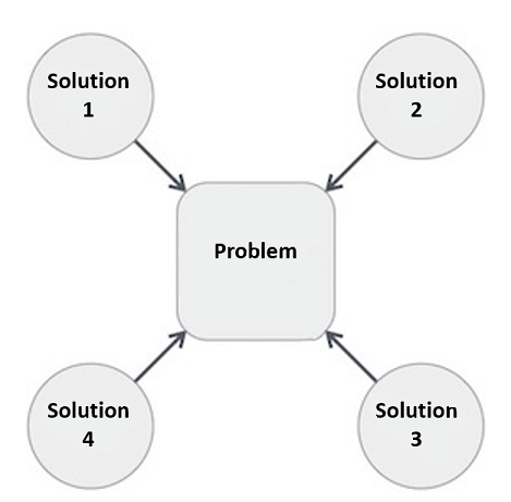
Hence, many solution algorithms can be derived for a given problem. The next step is to analyze those proposed solution algorithms and implement the best suitable solution.
Notes On Big-O Notation
-
We use big-O notation in the analysis of algorithms to describe an algorithm’s usage of computational resources in a way that is independent of computer architecture or clock rate.
-
The worst case running time, or memory usage, of an algorithm is often expressed as a function of the length of its input using big O notation.
- We generally seek to analyze the worst-case running time. However it is not unusual to see a big-O analysis of memory usage.
- An expression in big-O notation is expressed as a capital letter “O”, followed by a function (generally) in terms of the variable n, which is understood to be the size of the input to the function you are analyzing.
- This looks like: O(n).
- If we see a statement such as: f(x) is O(n) it can be read as “f of x is big Oh of n”; it is understood, then, that the number of steps to run f(x) is linear with respect to |x|, the size of the input x.
- A description of a function in terms of big O notation only provides an upper bound on the growth rate of the function.
- This means that a function that is O(n) is also, technically, O(n^2 ), O(n^3 ), etc
- However, we generally seek to provide the tightest possible bound. If you say an algorithm is O(n^3 ), but it is also O(n^2 ), it is generally best to say O(n^2 ).
- Why do we use big-O notation? Big-O notation allows us to compare different approaches for solving problems and predict how long it might take to run an algorithm on a very large input.
- With big-O notation we are particularly concerned with the scalability of our functions. Big-O bounds may not reveal the fastest algorithm for small inputs (for example, remember that for x < 0.5, x^3 < x^2 ) but will accurately predict the long-term behavior of the algorithm.
- This is particularly important in the realm of scientific computing: for example, doing analysis on the human genome or data from the Hubble telescope involves input (arrays or lists) of sizes well into the tens of millions (of base pairs, pixels, etc).
1
- At this scale it becomes easy to see why big O notation is helpful. Say you’re running a program to analyze base pairs and have two different implementations: one is O(n lg n) and the other is O(n^3 ). Even without knowing how fast of a computer you’re using, it’s easy to see that the first algorithm will be n^3 /(n lg n) = n^2 / lg n faster than the second, which is a BIG difference at input that size.
Big-O notation is widespread wherever we talk about algorithms. If you take any Courseclasses in the future, or do anything involving algorithms in the future, you will run into big-O notation again.
-
Some common bounds you may see, in order from smallest to largest:
-
O( 1 ): Constant time. O( 1 ) = O( 10 ) = O( 2100 ) - why? Even though the constants are huge, they are still constant. Thus if you have an algorithm that takes 2100 discreet steps, regardless of the size of the input, the algorithm is still O( 1 ) - it runs in constant time; it is not dependent upon the size of the input.
-
O(lg n): Logarithmic time. This is faster than linear time; O(log 10 n) = O(ln n) = O(lg n) (traditionally in Computer Science we are most concerned with lg n, which is the base-2 logarithm – why is this the case?). The fastest time bound for search.
-
O(n): Linear time. Usually something when you need to examine every single bit of your input.
-
O(n lg n): This is the fastest time bound we can currently achieve for sorting a list of elements.
-
O(n^2 ): Quadratic time. Often this is the bound when we have nested loops.
-
O( 2^n): Really, REALLY big! A number raised to the power of n is slower than n raised to any power.
-
-
Some questions for you:
- Does O(100n^2 ) = O(n^2 )?
- Does O(^14 n^3 ) = O(n^3 )?
- Does O(n) + O(n) = O(n)?
The answers to all of these are Yes! Why? big-O notation is concerned with the long-term, or limiting, behavior of functions. If you’re familiar with limits, this will make sense - recall that lim x^2 = lim 100x^2 = ∞ x→∞ x→∞
Basically, go out far enough and we can’t see a distinction between 100x^2 and x^2. So, when we talk about big-O notation, we always drop coefficient multipliers - because they don’t make a difference. Thus, if you’re analysing your function and you get that it is O(n) + O(n), that doesn’t equal O(2n) - we simply say it is O(n).
2
One more question for you: Does O(100n^2 + 41 n^3 ) = O(n^3 )? Again, the answer to this is Yes! Because we are only concerned with how our algorithm behaves for very large values of n, when n is big enough, the n^3 term will always dominate the n^2 term, regardless of the coefficient on either of them. In general, you will always say a function is big-O of its largest factor - for example, if something is O(n^2 + n lg n + 100 ) we say it is O(n^2 ). Constant terms, no matter how huge, are always dropped if a variable term is present - so O( 800 lg n + 73891 ) = O(lg n), while O( 73891 ) by itself, with no variable terms present, is O( 1 ).
Now you should understand the What and the Why of big-O notation, as well as How we describe something in big-O terms. But How do we get the bounds in the first place?? Let’s go through some examples.
- We consider all mathematical operations to be constant time (O( 1 )) operations. So the following functions are all considered to be O( 1 ) in complexity:
def inc(x):
return x+
def mul(x, y):
return x*y
def foo(x):
y = x*77.
return x/8.
def bar(x, y):
z = x + y
w = x * y
q = (w**z) % 870

return 9*q
3
- Functions containing for loops that go through the whole input are generally O(n). For example, above we defined a function mul that was constant-time as it used the built-in Python operator *. If we define our own multiplication function that doesn’t use *, it will not be O( 1 ) anymore:
def mul2(x, y):
result = 0

for i in range(y):
result += x
return result
Here, this function is O(y) - the way we’ve defined it is dependent on the size of the input y, because we execute the for loop y times, and each time through the for loop we execute a constant-time operation.
- Consider the following code:
def factorial(n):
result = 1

for num in range(1, n+1):
result *= num
return num
What is the big-O bound on factorial?
- Consider the following code:
def factorial2(n):
result = 1

count = 0

for num in range(1, n+1):
result *= num
count += 1

return num
What is the big-O bound on factorial2
4
- The complexity of conditionals depends on what the condition is. The complexity of the condition can be constant, linear, or even worse - it all depends on what the condition is.
def count_ts(a_str):
count = 0
for char in a_str:
if char == ’t’:
count += 1

return count
In this example, we used an if statement. The analysis of the runtime of a conditional is highly dependent upon what the conditional’s condition actually is; checking if one character is equal to another is a constant-time operation, so this example is linear with respect to the size of a str. So, if we let n = |a str|, this function is O(n).
Now consider this code:
def count_same_ltrs(a_str, b_str):
count = 0

for char in a_str:
if char in b_str:
count += 1

return count
-
This code looks very similar to the function count_ts, but it is actually very different! The conditional checks if char in b str - this check requires us, in the worst case, to check every single character in b str! Why do we care about the worst case? Because big-O notation is an upper bound on the worst-case running time. Sometimes analysis becomes easier if you ask yourself, what input could I give this to achieve the maximum number of steps? For the conditional, the worst-case occurs when char is not in b str
-
Then we have to look at every letter in b str before we can return False. So, what is the complexity of this function? Let n = |a str| and m = |b str|. Then, the for loop is O(n). Each iteration of the for loop executes a conditional check that is, in the worst case, O(m). Since we execute an O(m) check O(n) time, we say this function is O(nm).
5
- While loops: With while loops you have to combine the analysis of a conditional with one of a for loop.
def factorial3(n):
result = 1

while n > 0:
result *= n
n -= 1

return result
What is the complexity of factorial3
def char_split(a_str):
result = []
index = 0

while len(a_str) != len(result):
result.append(a_str[index])
index += 1

return result
- In Python, len is a constant-time operation. So is string indexing (this is because strings are immutable) and list appending. So, what is the time complexity of char split? If you are curious, there is a little more information on Python operator complexity here: http://wiki.python.org/moin/TimeComplexity
Note:
-
CPython just means “Python written in the C language”. You are actually using CPython.
-
If you are asked to find the worst-case complexity, you want to use the Worst Case bounds.
-
Note that operations such as slicing and copying aren’t O( 1 ) operations.
-
Nested for loops - anytime you’re dealing with nested loops, work from the inside out. Figure out the complexity of the innermost loop, then go out a level and multiply (this is similar to the second piece of code in Example 5). So, what is the time complexity of this code fragment, if we let n = |z|?
result = 0

for i in range(z):
for j in range(z):
result += (i*j)
6
Recursion. Recursion can be tricky to figure out; think of recursion like a tree. If the tree has lots of branches, it will be more complex than one that has very few branches. Consider recursive factorial:
def r_factorial(n):
if n <= 0:
return 1

else:
return n*r_factorial(n-1)
What is the time complexity of this? The time complexity of r factorial will be dependent upon the number of times it is called. If we look at the recursive call, we notice that it is: r factorial(n-1). This means that, every time we call r factorial, we make a recursive call to a subproblem of size n − 1. So given an input of size n, we make the recursive call to subproblem of size n − 1 , which makes a call to subproblem of size n − 2 , which makes a call to subproblem of size n − 3 ,... see a pattern? We’ll have to do this until we make a call to n − n = 0 before we hit the base case - or, n calls. So, r factorial is O(n). There is a direct correlation from this recursive call to the iterative loop for i in range(n, 0, -1). In general, we can say that any recursive function g(x) whose recursive call is on a subproblem of size x − 1 will have a linear time bound, assuming that the rest of the recursive call is O( 1 ) in complexity (this was the case here, because the n* factor was O( 1 )).
**How about this function?
def foo(n):
if n <= 1:
return 1

return foo(n/2) + 1
In this problem, the recursive call is to a subproblem of size n/2. How can we visualize this? First we make a call to a problem of size n, which calls a subproblem of size n/2, which calls a subproblem of size n/4, which calls a subproblem of size n/( 23 ),... See the pattern yet? We can make the intuition that we’ll need to make recursive calls until n = 1 , which will happen when n/2x^ = 1.
So, to figure out how many steps this takes, simply solve for x in terms of n:
n
= 1
2 x^
n = 2 x^
log 2 n = log 2 ( 2 x)
∴ x = log 2 n
7
So, it’ll take log 2 n steps to solve this recursive equation. In general, we can say that if a recursive function g(x) makes a recursive call to a subproblem of size x/b, the complexity of the function will be logbn. Again, this is assuming that the remainder of the recursive function has complexity of O( 1 ).
Finally, how do we deal with the complexity of something like Fibonacci? The recursive call to Fibonacci is fib(n) = fib(n − 1 ) + fib(n − 2 ).
This may initially seem linear, but it’s not. If you draw this in a tree fashion, you get something like:
The depth of this tree (the number of levels it has) is n, and at each level we see a branching factor of two (every call to fib generates two more calls to fib). Thus, a loose bound on fib is O( 2 n). In fact, there exists a tighter bound on Fibonacci involving the Golden Ratio; Google for “Fibonacci complexity” to find out more if you’re interested in maths : D
Introduction to Algorithms
Objectives
In this chapter, you will:
- Understand why algorithm analysis is important
- Use "Big-O" to describe execution time
- Understand the "Big-O" execution time of common operations on Python lists and dictionaries
- Understand how the implementation of Python data impacts algorithm analysis
- Understand how to benchmark simple Python programs
Demonstration Labs
Algorithms Demo 1:
File: timing1.py
Prints the running times for problem sizes that double,
using a single loop.
problemSize = 10000000
range_size = 5
print()
print("Count  Problem Size   Seconds")
work = 1
for count in range(range_size): #O(5n)
    start = time.time()         #O(1)
    #the start of the algorithm
    work = 1
    for x in range(problemSize): #O(n)
        work += 1 #O(2) = O(1) because of limits
        work -= 1 #O(2) = O(1) because of limits
    #the end of the algorithm
    elapsed = time.time() - start
    print(count+1     , end='')
    print("%12d%16.3f" % (problemSize, elapsed))
    problemSize *= 2
Expected Output:
| Problem Size | Seconds |
|---|---|
| 10000000 | 3.8 |
| 20000000 | 7.591 |
| 40000000 | 15.352 |
| 80000000 | 30.697 |
| 160000000 | 61.631 |
Algorithms Demo 2
Timing2.py
As another example, consider the following change in tester program's algorithm:
import time

problemSize = 1000

for count in range(5): #O(5n)
    start = time.time() #O(1)
    #start the algorithm
    work = 1
    for j in range(problemSize): # O(n)
        for k in range(problemSize):
            work += 1 #O(2)
            work -= 1 #O(2)
    #end of algorithm
    elapsed = time.time() - start

    print(f'{count+1}  {problemSize} - {elapsed}')
    problemSize *= 2
Expected Output:
| PROBLEM SIZE | SECONDS |
|---|---|
| 1000 | 0.387 |
| 2000 | 1.581 |
| 4000 | 6.463 |
| 8000 | 25.702 |
| 16000 | 102.666 |
Algorithms Demo 3:
File: counting.py
Prints the number of iterations for problem sizes
that double, using a nested loop.
problemSize = 1000
range_size = 5
print("Count  Problem Size     Iterations")

for count in range(range_size):
    number = 0

    work = 1
    for j in range(problemSize):
        for k in range(problemSize):
            number += 1
            work += 1
            work -= 1

    print(count+1   , end="")
    print("%12d%15d" % (problemSize, number))
    problemSize *= 2
**As you can see from the results, the number of iterations is the square of the problem size
Expected Output:
| PROBLEM SIZE | SECONDS |
|---|---|
| 1000 | 1000000 |
| 2000 | 4000000 |
| 4000 | 16000000 |
| 8000 | 64000000 |
| 16000 | 256000000 |
Algorithms Demo 4:
File: countfib.py Prints the number of calls of a recursive Fibonacci function with problem sizes that double.
from collections import Counter

def fib(n, counter):
    #count the number of calls of fib function
    counter[n] += 1
    if n < 3:
        return 1 #base case
    else:
        return fib(n-1, counter) + fib(n-2, counter)

problemSize = 2
for count in range(5):
    counter = Counter()
    #start of the algorithm
    fib(problemSize, counter)
    #end algorithm
    print(f'{problemSize}   {counter}')
    problemSize *= 2
Expected Output:
| PROBLEM SIZE | CALLS |
|---|---|
| 2 | 1 |
| 4 | 5 |
| 8 | 41 |
| 16 | 1973 |
| 32 | 4356617 |
Search Algorithms
Minimum Example Search
def index0fmin(lyst):
    """Returns the index of the minimum item."""
    minIndex = 0
    currentIndex = 1
    while currentIndex =1
        if lyst[currentIndex] < lyst[minIndex]:
            minIdex = currentIndex
        currentIndex += 1
    return minIndex
Sequential Search of List
def sequentialSearch(target, lyst):
    """Returns the position of the target item if found, or -1 otherwise."""
    position = 0
    while position < len(lyst):
        if target == lyst[position]:
            return position
        position += 1
    return -1
Binary Search:
def binarySearch(target, sortedLyst):
    left = 0
    right = len(sortedLyst) - 1
    while left <= right:
        midpoint = (left + right) // 2
        if target == sortedLyst[midpoint]:
            return midpoint
        elif target < sortedLyst[midpoint]:
            right = midpoint - 1
        else:
            left = midpoint + 1
        return -1
Comparing Data Items
class SavingsAccount(object):
    """This class represents a savings account with the owner's nmae, PIN, and balance."""
    def _init_(self, name, pin, balance = 0.0):
        self.name = name
        self.pin = pin
        self.balance = balance

    def _lt_(self, other):
        return self.name < other.name

    # Other methods, including _eq_

>>> s1 = SavingsAccount("Ken", "1000", 0)
>>> s2 = SavingsAccount("Bill", "1001", 30)
>>> s1 < s2
False
>>> s2 < s1
True
>>> s1 > s2
True
>>> s2 > s1
False
>>> s2 == s1
False
>>> s3 = SavingsAccount("Ken", "1000", 0)
>>> s1 == s3
True
>>> s4 = s1
>>> s4 == s1
True
- You can now place the accounts in a list and sort them by name.
Sort Algorithms
Basic Sort Demo 1:
def swap(lyst, i, j):
    """Exchanges the items at positions i and j."""
    # You could say lyst[i], lyst[j] = lyst[j]. lyst[i]
    # but the following code shows what is really going on
    temp = lyst[i]
    lyst[i] = lyst[j]
    lyst[j] = temp
Selection Sort Algorithm
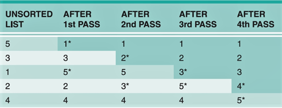
def selectionSort(lyst):
    i =0
    while i < len(lyst) - 1:     # Do n - 1 searches
        minIndex = i             # for the smallest
        j = i + 1
        while j < len(lyst):     # Start a search
            if lyst[j] < lyst[minIndex]:
                minIndex = j
            j += 1
        if minIndex != 1:        # Exchange if needed
            swap(lyst, minIndex, i)
        i += 1
Bubble Sort Algorithms
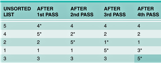
def bubbleSort(lyst):
    n = len(lyst)
    while n > 1:                       # Do n - 1 bubbles
        i = 1                          # Start each bubble
        while i < n:
            if lyst[i] < lyst[i - 1]:  # Exchange if needed
                swap(lyst, i, i - 1)
            i += 1
        n -= 1
Modified Bubble Sort function:
def bubbleSortWithTweak(lyst):
    n = len(lyst)
    while n< 1:
        swapped = False
        i = 1
        while i < n:
            if lyst[i] < lyst[i - 1]:  # Exchane if needed
                swap(lyst, i, i - 1)
                swapped = True
            i += 1
        if not swapped: return         # Return if no swaps
        n -= 1
Insertion Sort Algorithms
def insertionSort(lyst):
    i = l
    while i < len(lyst):
        itemToInsert = lsyt[i]
        j = i - 1
        while j >= 0:
            if itemToInsert < lyst[j]:
                lyst[j + 1] = lyst[j]
                j -= 1
            else:
                break
       lyst[j + 1] = itemToInsert
       i += 1
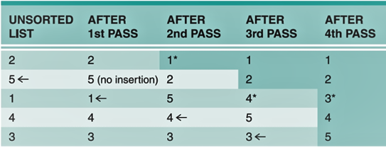
Quick Sort & Merge Sort Algorithms
Quicksort:

Implementation of Quicksort
def quicksort(lyst):
    quicksortHelper(lyst, 0, len(lyst) - 1)

def quicksortHelper(lyst, left, right):
    if left < right:
        pivotLocation = partition(lyst, left, right)
        quicksortHelper(lyst, left, pivotlLocation - 1)
        quicksortHelper(lyst, pivotLocation + 1, right)

def partition(lyst, left, right):
    # Find the pivot and exchange it with the last item
    middle = (left + right) // 2
    pivot = lyst[middle]
    lyst[middle] = lyst[right]
    lyst[right] = pivot
    # Set boundary point to first position
    boundry = left
    # Move items less than pivot to the left
    for index in range(left, right):
        if lyst[index] < pivot:
            swap(lyst, index, boundary)
            boundary += 1
    # Exchange the pivot item and the boundary item
    swap (lyst, right, boundary)
    return boundary

# Earlier definition of the swap function goes here

import random

def main(size = 20, sort = quicksort):
    lyst = []
    for count in range(size):
        lyst.append(random.randint(1, size + 1))
    print(lyst)
    sort(lyst)
    print(lyst)

if _namd_ == "_main_":
    main()
Merge Sort Examples
from arrays import Array

def mergeSort(lyst):
    # lyst     list being sorted
    # copyBuffer temporary space needed during merge
    copyBuffer = Array(len(lyst))
    mergeSortHelper(lyst, copyBuffer, 0, len(lyst) - 1)
from arrays import Array

def mergeSort(lyst):
    # lyst     list being sorted
    # copyBuffer temporary space needed during merge
    copyBuffer = Array(len(lyst))
    mergeSortHelper(lyst, copyBuffer, 0, len(lyst) - 1)
def mergeSortHelper(lyst, copyBuffer, low, high):
    # lyst          list being sorted
    # copyBuffer    temp space needed during merge
    # low, high     bounds of sublist
    # middle        midpoint of sublist
    if low < high:
        middle = (low + high) // 2
        mergeSortHelper(lyst, copyBuffer, low, middle)
        mergeSortHelper(lyst, copyBuffer, middle + 1, high)
        merge(lyst, copyBuffer, low, middle, high)
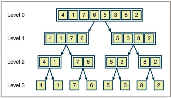
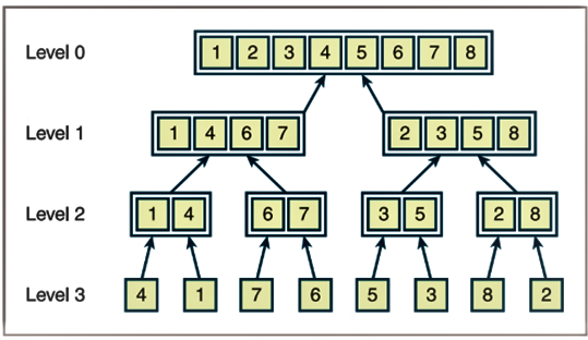
def merge(lyst, copyBuffer, low, middle, high):
# lyst list that is being sorted
# copyBuffer temp space needed during the merge process
# low beginning of first sorted sublist
# middle end of first sorted sublist
# middle + 1 beginning of second sorted sublist
# high end of second sorted sublist
# Initialize i1 and i2 to the first itend of second sorted sublist
i1 = low
i2 = middle + 1
# Interleave items forom the sublists into the copyBuffer in such a way that order is maintained
for i in range(low, high +1):
if i1 > middle:
copyBuffer[i] = lyst[i2] # First sublist exhausted
i2 += 1
elif i2 > high:
copyBuffer[i] = lyst[i1] # Second sublist exhausted
i1 += 1
elif lyst[i1] < lyst[i2]
copyBuffer[i] = lyst[i1] # Item in first sublist <
i1 += 1
else:
copyBuffer[i] = lyst[i2] # Item in second sublist <
i2 += 1
for i in range (low, high + 1): # Copy sorted items back to proper position in lyst
lyst[i] = copyBuffer[i] # proper position in lyst
Practice Labs
Complexity Exercises
Exercise 1
- Write a tester program that counts and displays the number of iterations of the following loop:
while problemSize > 0:
problemSize = problemSize // 2
Exercise 2
- Run the program you created in Exercise 1 using problem sizes, of 1000, 2000, 4000, 10,000, and 100,000. As the problem size doubles or increases by a factor of 10.
What happens to the number iterations?
Exercise 3
- The difference between the results of two calls of the functions time.time() is an elapsed time. Because the operating system might use the CPU for part of this time, the elapsed time might not reflect the actual time that a Python code segment uses the CPU. Browse the Python documention for an alternative way of recording the processing time, and describe how this would be done.
Exercise 4
- Assume that each of the following expressions indicates the number of operations performed by an algorithm for a problem size of n. Point out the dominant term of each algorithm and use big-O notation to classify it.
a. 2^n - 4n^2 + 5n
b. 3n^2 + 6
c. n^3 + n^2 - n
Exercise 5
- For problem size n, algorithms A and B perform n^2 and (1/2)n^2 + (1/2)n instructions, respectively. Which algorithm does more work? Are there particular problem sizes for which one algorithm performs significantly better than the other? Are there particular problem sizes for which both algorithms perform approximately the same amount of work?
Exercises 6
- At what point does an n^4 algorithm begin to perform better than a 2^n algorithm?
Sort Exercises
-
Describe the strategy of quicksort and explain why it can reduce the time complexity of sorting from O(n2) to O(n log n).
-
Why is quicksort not O(n log n) in all cases? Describe the worst-case situation for quicksort and give a list of 10 integers, 1- 10, that would produce this behavior.
-
The partition operation in quicksort chooses the item at the midpoint as the pivot. Describe two other strategies for selecting a pivot value.
-
Sandra has a bright idea: when the length of a sublist in quicksort is less than a certain number - say, 30 elements - run an insertion sort to process that sublist.
Explain why this is a bright idea. -
Why is merge sort an O(n log n) algorithm in the worst case?
Searching is integral to life - We search for things all the time; or at least I do! As often is the case, just as it is in life, so it is in computer science and searching plays a very important role when it comes to working with data. A search algorithm is any algorithm which solves the Search problem, namely, to retrieve information stored within some data structure, or calculated in the search space of a problem domain. Examples of such structures include but are not limited to a Linked List, an Array data structure, or a Search tree. The appropriate search algorithm often depends on the data structure being searched, but also on any a priori knowledge about the data. Searching also encompasses algorithms that query the data structure, such as the SQL SELECT command.
Linear Search Algorithm
The _Linear Search a_lgorithm is a simple algorithm, where each item in the list (starting from the first item) is investigated until the required item is found, or the end of the list is reached.
The Linear Search algorithm is implemented in Python as follows:
def linearSearch(item, my_list):
found = False
position = 0
while position < len(my_list) and not found:
if my_list[position] == item:
found = True
position = position + 1
return found
Let's test the code. Enter the following statement at the end of the Python script above:
bag = ['book', 'pencil', 'pen', 'note book', 'sharpener', 'eraser']
item = input('What item do you want to check for in the bag?')
itemFound = linearSearch(item, bag)
if itemFound:
print ('Yes, the item is in the bag')
else:
print ('Oops, your item seems not to be in the bag')
When you enter the input, make sure it is between single or double quotes (i.e. 'pencil'). If you input 'pencil', for instance, you should get the following output:
Yes, the item is in the bag
Whereas, if you enter 'ruler' as input, you will get the following output:
Oops, your item seems not to be in the bag
As we can see, Python proves itself again to be a programming language that makes it easy to program algorithmic concepts as we did here, dealing with sorting and searching algorithms.
It is important to note that there are other types of sorting and searching algorithms.
Binary Search
Given a sorted array arr[] of n elements, write a function to search a given element x in arr[].
A simple approach is to do linear search . The time complexity of above algorithm is O(n). Another approach to perform the same task is using Binary Search.
Binary Search: Search a sorted array by repeatedly dividing the search interval in half. Begin with an interval covering the whole array. If the value of the search key is less than the item in the middle of the interval, narrow the interval to the lower half. Otherwise narrow it to the upper half. Repeatedly check until the value is found or the interval is empty.
Binary Search
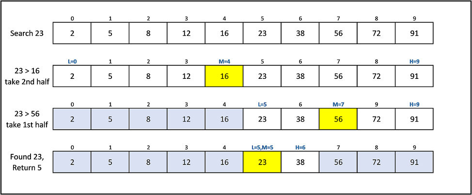
The idea of binary search is to use the information that the array is sorted and reduce the time complexity to O(Log n).
We basically ignore half of the elements just after one comparison.
- Compare x with the middle element.
- If x matches with middle element, we return the mid index.
- Else If x is greater than the mid element, then x can only lie in right half subarray after the mid element. So we recur for right half.
- Else (x is smaller) recur for the left half.
Sorting Algorithms
Objectives
Sorting refers to arranging data in a particular format. Sorting algorithm specifies the way to arrange data in a particular order. Most common orders are in numerical or lexicographical order.
The importance of sorting lies in the fact that data searching can be optimized to a very high level, if data is stored in a sorted manner. Sorting is also used to represent data in more readable formats. Below we see five such implementations of sorting in python.
- Bubble Sort
- Merge Sort
- Insertion Sort
- Shell Sort
- Selection Sort
Bubble Sort
It is a comparison-based algorithm in which each pair of adjacent elements is compared and the elements are swapped if they are not in order.
def bubblesort(list):
Swap the elements to arrange in order
for iter\_num in range(len(list) -1, 0, -1):
for idx in range(iter\_num):
if list[idx] \> list[idx+1]:
temp = list[idx]
list[idx] = list[idx+1]
list[idx+1] = temp
list =[19,2,31,45,6,11,121,27]
bubblesort(list)
print(list)
When the above code is executed, it produces the following result:
[2,6,11,19,27,31,45,121]
Write a Python program to sort a list of elements using the bubble sort algorithm.
Note: According to Wikipedia "Bubble sort, sometimes referred to as sinking sort, is a simple sorting algorithm that repeatedly steps through the list to be sorted, compares each pair of adjacent items and swaps them if they are in the wrong order. The pass through the list is repeated until no swaps are needed, which indicates that the list is sorted. The algorithm, which is a comparison sort, is named for the way smaller elements "bubble" to the top of the list. Although the algorithm is simple, it is too slow and impractical for most problems even when compared to insertion sort. It can be practical if the input is usually in sort order but may occasionally have some out-of-order elements nearly in position.
Step by step pictorial presentation:
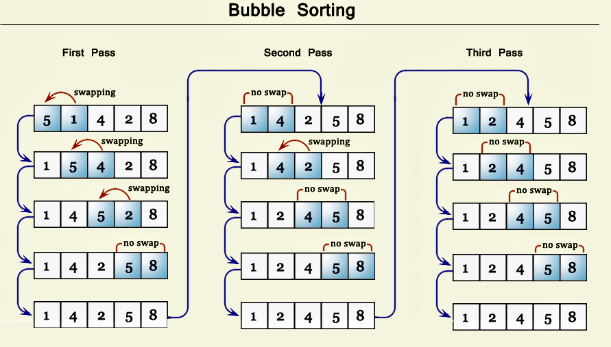
Merge Sort
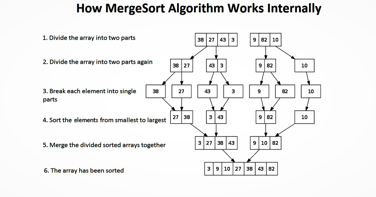
Merge sort divides the array into equal halves and then combines them in a sorted manner
def merge\_sort(unsorted\_list):
if len(unsorted\_list)\<=1:
return unsorted\_list
Find the middle point and devide it
middle = len(unsorted\_list)// 2
left\_list = unsorted\_list[:middle]
right\_list = unsorted\_list[middle:]
left\_list = merge\_sort(left\_list)
right\_list = merge\_sort(right\_list)
return list(merge(left\_list, right\_list))
Merge the sorted halves
def merge(left\_half,right\_half):
res =[]
while len(left\_half)!= 0 and len(right\_half)!= 0:
if left\_half[0]\< right\_half[0]:
res.append(left\_half[0])
left\_half.remove(left\_half[0])
else:
res.append(right\_half[0])
right\_half.remove(right\_half[0])
if len(left\_half) == 0:
res = res + right\_half
else:
res = res + left\_half
return res
unsorted\_list =[64,34,25,12,22,11,90]
print(merge\_sort(unsorted\_list))
When the above code is executed, it produces the following result:
[11,12,22,25,34,64,90]
Insertion Sort
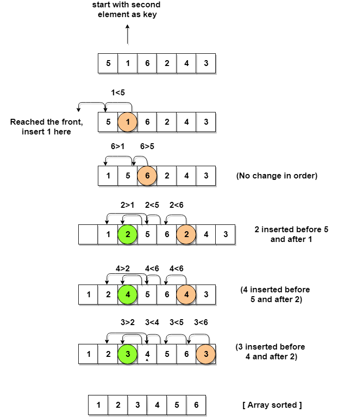
Insertion sort involves finding the right place for a given element in a sorted list. So in beginning we compare the first two elements and sort them by comparing them. Then we pick the third element and find its proper position among the previous two sorted elements. This way we gradually go on adding more elements to the already sorted list by putting them in their proper position.
def insertion\_sort(InputList):
for i in range(1, len(InputList)):
j = i-1
nxt\_element =InputList[i]
# Compare the current element with next one
while(InputList[j]\> nxt\_element)and(j\> = 0):
InputList[j+1] =InputList[j]
j = j-1
InputList[j+1] = nxt\_element
list = [19,2,31,45,30,11,121,27]
insertion\_sort(list)
print(list)
When the above code is executed, it produces the following result:
[2,11,19,27,30,31,45,121]
Shell Sort
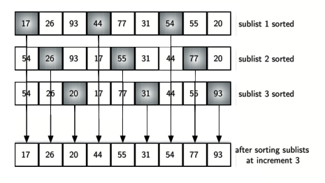
Shell Sort involves sorting elements which are away from ech other. We sort a large sublist of a given list and go on reducing the size of the list until all elements are sorted. The below program finds the gap by equating it to half of the length of the list size and then starts sorting all elements in it. Then we keep resetting the gap until the entire list is sorted.
def shellSort(input\_list):
gap = len(input\_list)// 2
while gap \>0:
for i in range(gap, len(input\_list)):
temp = input\_list[i]
j = i
# Sort the sub list for this gap
while j \> = gap and input\_list[j - gap]\> temp:
input\_list[j] = input\_list[j - gap]
j = j-gap
input\_list[j] = temp
# Reduce the gap for the next element
gap = gap//2
list =[19,2,31,45,30,11,121,27]
shellSort(list)
print(list)
When the above code is executed, it produces the following result:
[2,11,19,27,30,31,45,121]
Selection Sort
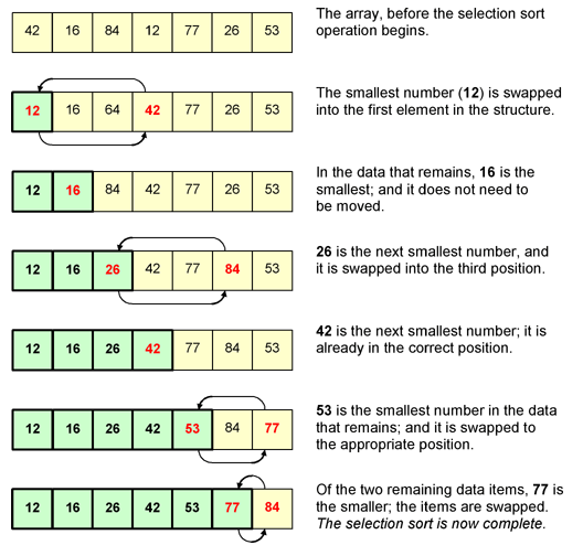
In selection sort we start by finding the minimum value in a given list and move it to a sorted list. Then we repeat the process for each of the remaining elements in the unsorted list. The next element entering the sorted list is compared with the existing elements and placed at its correct position. So at the end all the elements from the unsorted list are sorted.
def selection\_sort(input\_list):
for idx in range(len(input\_list)):
min\_idx = idx
for j in range( idx +1, len(input\_list)):
if input\_list[min\_idx]\> input\_list[j]:
min\_idx = j
Swap the minimum value with the compared value
input\_list[idx], input\_list[min\_idx]= input\_list[min\_idx], input\_list[idx]
l =[19,2,31,45,30,11,121,27]
selection\_sort(l)
print(l)
When the above code is executed, it produces the following result:
[2,11,19,27,30,31,45,121]
Intro to Data Structures in Python
Introduction:
In this section, the students will learn to implement complex data structures using Python
Recognizing more advanced data structures allow for more efficient storage, organization, and access of data.
This section will introduce and review the use of more advanced data structures in Python. Recognizing more advanced (higher and lower) methods for manipulating data will allow the creation of more effective and appropriately designed applications.
Topics Covered:
To access the Data Structures' slides please click here
Lesson Objectives:
- LO 1 Identify and implement advanced data structures in Python (Proficiency Level: B)
- MSB 1.1 Identify types and uses of linked lists in Python (Proficiency Level: B)
- MSB 1.2 Identify queue and stack structures in Python (Proficiency Level: B)
- MSB 1.3 Identify the use cases for tree structures in Python (Proficiency Level: B)
Performance Objectives (Proficiency Level: 3c)
-
Conditions: Given access to (references, tools, etc.):
- Access to specified remote virtual environment
- Student Guide and Lab Guide
- Student Notes
-
Performance/Behavior Tasks:
- Implement linked lists in Python
- Use stack functions in Python
- Implement binary tree traversal in Python
-
Standard(s)
- Criteria: Demonstration: Correctable to 100% in class
- Evaluation: Students will have 4 hours to complete the timed evaluation consisting of both cognitive and performance components.
- Minimum passing score is 80%
Lists and Pointer Structures
Objectives
By the end of this lesson topic you should:
- Understand pointers in Python
- Treating the concept of nodes
- Implementing singly, doubly, and circularly linked lists
Introduction
At this point in training you will have already seen lists in Python. They are convenient and powerful. Normally, any time you need to store something in a list, you use Python's built-in list implementation. In this chapter, however, we are more interested in understanding how lists work. So we are going to study list internals. As you will notice, there are different types of lists.
Python's list implementation is designed to be powerful and to encompass several different use cases. We are going to be a bit more strict in our definition of what a list is. The concept of a node is very important to lists. We shall discuss them in this chapter, but this concept will, in different forms, come back throughout the rest of the book. In this lesson, we are going to deal quite a bit with pointers. So it may be useful to remind ourselves what these are.
Understanding Pointers in Python
To begin with, imagine that you have a house that you want to sell. Lacking time, you contact an agent to find interested buyers. So you pick up your house and take it over to the agent, who will in turn carry the house to anybody who may want to buy it. Ludicrous, you say? Now imagine that you have a few Python functions that work with images. So you pass high-resolution image data between your functions.
Of course, you don't carry your house around. What you would do is write the address of the house down on a piece of scrap paper and hand it over to the agent. The house remains where it is, but the note containing the directions to the house is passed around. You might even write it down on several pieces of paper. Each one is small enough to fit in your wallet, but they all point to the same house.
As it turns out, things are not very different in Python land. Those large image files remain in one single place in memory. What you do is create variables that hold the locations of those images in memory. These variables are small and can easily be passed around between different functions.
That is the big benefit of pointers: they allow you to point to a potentially large segment of memory with just a simple memory address.
Support for pointers exists in your computer's hardware, where it is known as indirect addressing.
In Python, you don't manipulate pointers directly, unlike in some other languages, such as C or Pascal. This has led some people to think that pointers aren't used in Python. Nothing could be further from the truth. Consider this assignment in the Python interactive shell:
>>> s = set()
We would normally say that s is a variable of the type set. That is, s is a set. This is not strictly true, however. The variable s is rather a reference (a "safe" pointer) to a set. The set constructor creates a set somewhere in memory and returns the memory location where that set starts. This is what gets stored in s.
Python hides this complexity from us. We can safely assume that s is a set and that everything works fine.
Arrays
An array is a sequential list of data. Being sequential means that each element is stored right after the previous one in memory. If your array is really big and you are low on memory, it could be impossible to find large enough storage to fit your entire array. This will lead to problems.
Of course, the flip side of the coin is that arrays are very fast. Since each element follows from the previous one in memory, there is no need to jump around between different memory locations. This can be a very important point to take into consideration when choosing between a list and an array in your own real-world applications.
Pointer structures
Contrary to arrays, pointer structures are lists of items that can be spread out in memory. This is because each item contains one or more links to other items in the structure. What type of links these are dependent on the type of structure we have. If we are dealing with linked lists, then we will have links to the next (and possibly previous) items in the structure. In the case of a tree, we have parent-child links as well as sibling links. In a tile-based game where the game map is built up of hexes, each node will have links to up to six adjacent map cells. There are several benefits with pointer structures. First of all, they don't require sequential storage space. Second, they can start small and grow arbitrarily as you add more nodes to the structure.
However, this comes at a cost. If you have a list of integers, each node is going to take up the space of an integer, as well as an additional integer for storing the pointer to the next node.
Singly Linked List
Objectives
- detailed understanding on what is a singly linked list
- Understand how singly linked list are used
- Understand basic operations that can be performed on singly linked lists
- Perform basic operations on singly linked lists
Prerequisites
Prior to this topic, you should have a basic understanding of:
- Python 3
- OOP concepts
- Basic understanding of the purpose of singly linked lists
Nodes
Before we get into the details of what singly lists are, we must learn what nodes are. This is because nodes are the building blocks of a linked list. A node consists of two parts:
Data part - contains the data Address part - this is pointer that points to location of the next node In a singly linked list, each node’s address part contains the information about the location of the next node. This forms a series of chain or links. The first node of the linked list is kept track by the head pointer. The last node points to None.
Let us see the following diagram to understand this better:
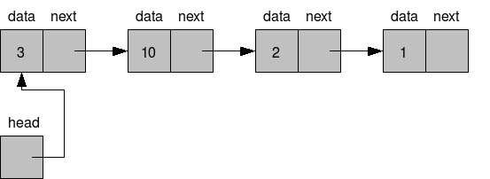
Note: In the above figure, the last element 1 points to None. Even though these nodes are drawn contiguous to each other, in reality, they may or may not be in contiguous memory locations.
Check out this animation for the visualization of the working of a linked list.
Tip: Always try to draw these data structures to get a clear understanding.
How to create a Singly Linked List? Creating classes Firstly, you must create a node in order to create a singly linked list. To do this, we create a class Node with data and nextNode attributes. As discussed earlier, the data attribute will contain the data and the nextNode will simply point to the next node in the linked list. We will make the default value of nextNode to be None. You can use getter and setter methods to do this.
Now that the Node class is created, it is time to create the LinkedList class. This has only one attribute, head. By default, this will point to None. If the head points to None it means that the linked list is empty. To keep track of the number of nodes in the linked list, we can add a size attribute to the LinkedList class and default it to 0.
Inserting a Node This is a method of the LinkedList class. Remember, to make the coding simple and efficient we will always add the new node to the beginning of the linked list. In other words, the head will always point to the most recently added node. If we add the new node to the end of the list, we need to do the extra work of finding the end of the list and then adding it. This is a wasteful operation. However, if you maintain another pointer, let’s call it the tail pointer such that it points to the last node, this can be done. You can insert a new node anywhere in the linked list. We have discussed the former approach i.e insertion at the beginning of the linked list.
Let’s say we need to add 7 to a linked list, we need to do the following steps:
Create a node object with 7 as the data and the next node pointing to head node Point the head pointer to this new node Finally, increment the size attribute by 1. It is always a good practice to return True if insertion was successful. This way the user knows what is happening.
Print Nodes This is a method of the LinkedList class. To print the data present in all the nodes of the linked list, we need to traverse one node at a time and print each node’s data part.
Coding a Singly Linked List
Class Node:
def _init_(self, data, nextNode = None):
self.data = data
self.nextNode = nextNode
def getData(self):
return self.data
def getNextNode(self):
return self.nextNode
def setNextNode(self, val):
self.nextNode = val
class LinkedList:
def _init_(self, head = None):
self.head = head
self.size = 0
def getSize(self):
return self.size
def addNode(self, data):
newNode = Node(data, self.head)
self.head = newNode
self.size+=1
return True
def printNode(self):
curr = self.head
while curr:
print(curr.data)
curr = curr.getNextNode()
myList = LinkedList()
print("Inserting")
print(myList.addNode(5))
print(myList.addNode(15))
print(myList.addNode(25))
print("Printing")
myList.printNode()
print("Size")
print(myList.getSize)
What are the advantages and disadvantages of Singly Linked Lists?
-
Advantages
- It’s a dynamic data structure in which insertion and deletion are simple as we don’t need to shift the elements. Just updating the next pointer will do the job for us.
- Stack and Queue data structures can be easily implemented using linked lists.
-
Disadvantages
- Additional memory is used up by the next pointers.
- Random access is not possible. You must traverse the linked list from the beginning to get to a particular node.
Summary
Throughout this topic we covered:
- Nodes
- What singly linked list are
- Some basic coding of a singly linked list
- Advantages of singly linked lists
- Disadvantages of singly linked lists
Doubly Linked List
Objectives
- Detailed understanding on what is a doubly linked list
- Understand how to create doubly linked lists
- Understand how to print all the nodes in a list
Creating a Double Linked List
Python program to create and display a doubly linked list.
In this program, we will create a doubly linked list and print all the nodes present in the list.
Doubly Linked List is a variation of the linked list. The linked list is a linear data structure which can be described as the collection of nodes. Nodes are connected through pointers. Each node contains two fields: data and pointer to the next field. The first node of the linked list is called the head, and the last node of the list is called the tail of the list.
One of the limitations of the singly linked list is that it can be traversed in only one direction that is forward. The doubly linked list has overcome this limitation by providing an additional pointer that points to the previous node. With the help of the previous pointer, the doubly linked list can be traversed in a backward direction thus making insertion and deletion operation easier to perform. So, a typical node in the doubly linked list consists of three fields:
Data represents the data value stored in the node. Previous represents a pointer that points to the previous node. Next represents a pointer that points to the next node in the list.
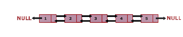
The above picture represents a doubly linked list in which each node has two pointers to point to previous and next node respectively. Here, node 1 represents the head of the list. The previous pointer of the head node will always point to NULL. Next pointer of node one will point to node 2. Node 5 represents the tail of the list whose previous pointer will point to node 4, and the next will point to NULL.
Algorithm:
Define a Node class which represents a node in the list. It will have three properties:
- data
- previous which will point to the previous node
- next which will point to the next node.
Define another class for creating a doubly linked list, and it has two nodes: head and tail.
Initially, head and tail will point to null.
addNode() will add node to the list:
It first checks whether the head is null, then it will insert the node as the head. Both head and tail will point to a newly added node. Head's previous pointer will point to null and tail's next pointer will point to null. If the head is not null, the new node will be inserted at the end of the list such that new node's previous pointer will point to tail. The new node will become the new tail. Tail's next pointer will point to null.
a. display() will show all the nodes present in the list.
Define a new node 'current' that will point to the head. Print current.data till current points to null. Current will point to the next node in the list in each iteration.
Program
#Represent a node of doubly linked list
class Node:
def _init_(self, data):
self.previous = None;
self.next = None;
class DoublyLinkedList:
# Represent the head and tail of the doubly linked list
def_init_(self):
self.head = None;
self.tail = None;
# If list is empty
if(self.head == None):
# Both head and tail will point to newNode
self.head = self.tail = newNode;
# head's previous will point to None
self.head.previous = None
# tail's next will pint to None, as it is the last node of the list
self.tail.next = None;
else:
# newNode will be added after tail such that tail's next will point to newNode
self.tail.next = newNode;
# newNode's previous will point to tail
newNode.previous = self.tail;
# newNode will become new tail
self.tail = newNode;
# As it is last node, tail's next will point to None
self.tail.next = None;
# display() will print out the nodes of the list
def display(self):
# Node current will point to head
current = self.head;
if(self.head == None):
print("list is empty");
return;
print("Nodes of doubly linked list: ");
while(current != None):
# Prints each node by incrementing pointer.
print(current.data);
current = current.next;
dList = DoublyLinkedList();
# Add nodes to the list
dList.addNode(1);
dList.addNode(2);
dList.addNode(3);
dList.addNode(4);
dList.addNode(5);
# Displays the nodes present in the list
dList.display();
Output: Nodes of doubly linked list: 1 2 3 4 5
Singly linked lists
A singly linked list is a list with only one pointer between two successive nodes. It can only be traversed in a single direction, that is, you can go from the first node in the list to the last node, but you cannot move from the last node to the first node.
We can actually use the node class that we created earlier to implement a very simple singly linked list:
>>> n1 = Node('eggs')
>>> n2 = Node('ham')
>>> n3 = Node('spam')
Next we link the nodes together so that they form a chain:
>>> n1.next = n2
>>> n2.next = n3
To traverse the list, you could do something like the following. We start by setting the variable current to the first item in the list:
current = n1
while current:
print(current.data)
current = current.next
In the loop we print out the current element after which we set current to point to the next element in the list. We keep doing this until we have reached the end of the list.
There are, however, several problems with this simplistic list implementation:
It requires too much manual work by the programmer It is too error-prone (this is a consequence of the first point) Too much of the inner workings of the list is exposed to the programmer We are going to address all these issues in the following sections.
Singly linked list class
A list is clearly a separate concept from a node. So we start by creating a very simple class to hold our list. We will start with a constructor that holds a reference to the very first node in the list. Since this list is initially empty, we will start by setting this reference to None:
class SinglyLinkedList:
def __init__(self):
self.tail = None
Append operation
The first operation that we need to perform is to append items to the list. This operation is sometimes called an insert operation. Here we get a chance to hide away the Node class. The user of our list class should really never have to interact with Node objects. These are purely for internal use.
A first shot at an append() method may look like this:
class SinglyLinkedList:
# ...
def append(self, data):
# Encapsulate the data in a Node
node = Node(data)
if self.tail == None:
self.tail = node
else:
current = self.tail
while current.next:
current = current.next
current.next = node
We encapsulate data in a node, so that it now has the next pointer attribute. From here we check if there are any existing nodes in the list (that is, does self.tail point to a Node). If there is none, we make the new node the first node of the list; otherwise, find the insertion point by traversing the list to the last node, updating the next pointer of the last node to the new node.
We can append a few items:
>>> words = SinglyLinkedList()
>>> words.append('egg')
>>> words.append('ham')
>>> words.append('spam')
List traversal will work more or less like before. You will get the first element of the list from the list itself:
>>> current = words.tail
>>> while current:
print(current.data)
current = current.next
A faster append operation
There is a big problem with the append method in the previous section: it has to traverse the entire list to find the insertion point. This may not be a problem when there are just a few items in the list, but wait until you need to add thousands of items. Each append will be slightly slower than the previous one. A O(n) goes to prove how slow our current implementation of the append method will actually be.
To fix this, we will store, not only a reference to the first node in the list, but also a reference to the last node. That way, we can quickly append a new node at the end of the list. The worst case running time of the append operation is now reduced from O(n) to O(1). All we have to do is make sure the previous last node points to the new node, that is about to be appended to the list. Here is our updated code:
class SinglyLinkedList:
def __init__(self):
# ...
self.tail = None
def append(self, data):
node = Node(data)
if self.head:
self.head.next = node
self.head = node
else:
self.tail = node
self.head = node
Take note of the convention being used. The point at which we append new nodes is through self.head. The self.tail variable points to the first node in the list.
Getting the size of the list
We would like to be able to get the size of the list by counting the number of nodes. One way we could do this is by traversing the entire list and increasing a counter as we go along:
def size(self):
count = 0
current = self.tail
while current:
count += 1
current = current.next
return count
This works, but list traversal is potentially an expensive operation that we should avoid when we can. So instead, we shall opt for another rewrite of the method. We add a size member to the SinglyLinkedList class, initializing it to 0 in the constructor. Then we increment size by one in the append method:
class SinglyLinkedList:
def __init__(self):
# ...
self.size = 0
def append(self, data):
# ...
self.size += 1
Because we are now only reading the size attribute of the node object, and not using a loop to count the number of nodes in the list, we get to reduce the worst case running time from O(n) to O(1).
Improving list traversal
If you notice how we traverse our list. That one place where we are still exposed to the node class. We need to use node.data to get the contents of the node and node.next to get the next node. But we mentioned earlier that client code should never need to interact with Node objects. We can achieve this by creating a method that returns a generator. It looks as follows:
def iter(self):
current = self.tail
while current:
val = current.data
current = current.next
yield val
Now list traversal is much simpler and looks a lot better as well. We can completely ignore the fact that there is anything called a Node outside of the list:
for word in words.iter():
print(word)
Notice that since the iter() method yields the data member of the node, our client code doesn't need to worry about that at all.
Deleting nodes
Another common operation that you would need to be able to do on a list is to delete nodes. This may seem simple, but we'd first have to decide how to select a node for deletion. Is it going to be by an index number or by the data the node contains? Here we will choose to delete a node by the data it contains.
The following is a figure of a special case considered when deleting a node from the list:
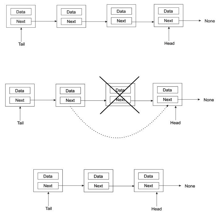
When we want to delete a node that is between two other nodes, all we have to do is make the previous node directly to the successor of its next node. That is, we simply cut the node to be deleted out of the chain as in the preceding image.
Here is the implementation of the delete() method may look like:
def delete(self, data):
current = self.tail
prev = self.tail
while current:
if current.data == data:
if current == self.tail:
self.tail = current.next
else:
prev.next = current.next
self.size -= 1
return
prev = current
current = current.next
It should take a O(n) to delete a node.
List search
We may also need a way to check whether a list contains an item. This method is fairly easy to implement thanks to the iter() method we previously wrote. Each pass of the loop compares the current data to the data being searched for. If a match is found, True is returned, or else False is returned:
def search(self, data):
for node in self.iter():
if data == node:
return True
return False
Clearing a list
We may want a quick way to clear a list. Fortunately for us, this is very simple. All we do is clear the pointers head and tail by setting them to None:
def clear(self):
""" Clear the entire list. """
self.tail = None
self.head = None
In one fell swoop, we orphan all the nodes at the tail and head pointers of the list. This has a ripple effect of orphaning all the nodes in between.
Performance Lab
- Complete the Linked List Performance Lab
Doubly Linked List Performance Lab
Create a Program to utilize a Doubly Linked List and involve Insertion, Deletion & Display Operations
This is a Python program to create a doubly linked list and implement insertion, deletion and display operations on the list.
Problem Description
The program creates a doubly linked list and presents the user with a menu to perform various operations on the list.
Problem Solution
- Create a class Node with instance variables data and next.
- Create a class DoublyLinkedList with instance variables first and last.
- The variable first points to the first element in the doubly linked list while last points to the last element.
- Define methods get_node, insert_after, insert_before, insert_at_beg, insert_at_end, remove and display.
- get_node takes an index as argument and traverses the list from the first node that many times to return the node at that index.
- The methods insert_after and insert_before insert a node after or before some reference node in the list.
- The methods insert_at_beg and insert_at_end insert a node at the first or last position of the list.
- The method remove takes a node as argument and removes it from the list.
- The method display traverses the list from the first node and prints the data of each node.
- Create an instance of DoublyLinkedList and present the user with a menu to perform operations on the list.
Please submit your work prior to continuing
Singly Linked List Lab
Create a Program to Check whether a Singly Linked List is a Palindrome
This is a Python program to check whether a singly linked list is a palindrome.
Problem Description
The program creates a linked list using data items input from the user and determines whether it is a palindrome.
Problem Solution
- Create a class Node with instance variables data and next.
- Create a class LinkedList with instance variables head and last_node.
- The variable head points to the first element in the linked list while last_node points to the last.
- Define methods append and display inside the class LinkedList to append data and display the linked list respectively.
- Define method get_prev_node which takes a reference node as argument and returns the node before it.
- Define a function is_palindrome which returns True if the linked list passed to it is a palindrome.
- The function is_palindrome iterates through the linked list from the start and the last node towards the middle to check if the list is a palindrome.
- Create an instance of LinkedList, append data to it and determine whether it is a palindrome.
Please submit your work before continuing
Stacks
A stack is a data structure that is often likened to a stack of plates. If you have just washed a plate, you put it on top of the stack. When you need a plate, you take it off the top of the stack. So the last plate to be added to the stack will be the first to be removed from the stack. Thus, a stack is a last in, first out (LIFO) structure:

The preceding figure depicts a stack of plates. Adding a plate to the pile is only possible by leaving that plate on top of the pile. To remove a plate from the pile of plates means to remove the plate that is on top of the pile.There are two primary operations that are done on stacks: push and pop. When an element is added to the top of the stack, it is pushed onto the stack. When an element is taken off the top of the stack, it is popped off the stack. Another operation which is used sometimes is peek, which makes it possible to see the element on the stack without popping it off.Stacks are used for a number of things. One very common usage for stacks is to keep track of the return address during function calls. Let's imagine that we have the following little program:
def b():
print('b')
def a():
b()
a()
print("done");
When the program execution gets to the call to a(), it first pushes the address of the following instruction onto the stack, then jumps to a. Inside a, b() is called, but before that, the return address is pushed onto the stack. Once in b() and the function is done, the return address is popped off the stack, which takes us back to a(). When a has completed, the return address is popped off the stack, which takes us back to the print statement.
Stacks are actually also used to pass data between functions. Say you have the following function call somewhere in your code:
somefunc(14, 'eggs', 'ham','spam')
What is going to happen is that 14, 'eggs', 'ham' and 'spam' will be pushed onto the stack, one at a time:

When the code jumps into the function, the values for a, b, c, d will be popped off the stack. The spam element will be popped off first and assigned to d, then "ham" will be assigned to c, and so on:
def somefunc(a, b, c, d):
print("function executed");
Stack implementation
Now let us study an implementation of a stack in Python. We start off by creating a node class, just as we did in the previous chapter with lists:
class Node:
def _init_(self, data = None):
self.data = data
self.next = None
This should be familiar to you by now: a node holds data and a reference to the next item in a list. We are going to implement a stack instead of a list, but the same principle of nodes linked together still applies.
Now let us look at the stack class. It starts off similar to a singly linked list. We need to know the node at the top of the stack. We would also like to keep track of the number of nodes in the stack. So we will add these fields to
class stack:
def _init_(self):
self.top = None
self.size = 0
Push operation
The push operation is used to add an element to the top of the stack. Here is an implementation:
def push(self, data):
node = Node(data)
if self.top:
node.next = self.top
self.top = node
else:
self.top = node
self.size += 1
In the following figure, there is no existing node after creating our new node. Thus self.top will point to this new node. The else part of the if statement guarantees that this happens:
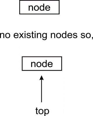
In a scenario where we have an existing stack, we move self.top so that it points to the newly created node. The newly created node must have its next pointer, pointing to the node that used to be the top node on the stack:
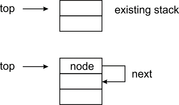
Pop operation
Now we need a pop method to remove the top element from the stack. As we do so, we need to return the topmost element as well. We will make the stack return None if there are no more elements:
def pop(self):
if self.top:
data = self.top.data
self.size -= 1
if self.top.next:
self.top = self.top.next
else:
self.top = None
return data
else:
return None
The thing to pay attention to here is the inner if statement. If the top node has its next attribute pointing to another node, then we must set the top of the stack to now point to that node:
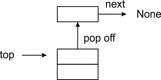
When there is only one node in the stack, the pop operation will proceed as follows:
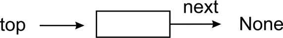
Removing such a node results in self.top pointing to None:
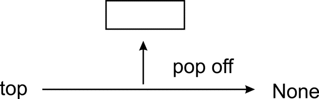
Peek
As we said earlier, we could also add a peek method. This will just return the top of the stack without removing it from the stack, allowing us to look at the top element without changing the stack itself. This operation is very straightforward. If there is a top element, return its data, otherwise return None (so that the behavior of peek matches that of pop):
def peek(self):
if self.top
return self.top.data
else:
return None
Bracket-matching application
Now let's look at an example of how we can use our stack implementation.
- We are going to write a little function that will verify whether a statement containing brackets--(, [, or {--is balanced, that is, whether the number of closing brackets matches the number of opening brackets.
It will also ensure that one pair of brackets really is contained in another:
def check_brackets(statement):
stack = Stack()
for ch in statement:
if ch in ('{', '[', '('):
stack.push(ch)
if ch in ('}', ']', ')'):
last = stack.pop()
if last is '{' and ch is '}':
continue
elif last is '[' and ch is ']':
continue
elif last is '(' and ch is ')':
continue
else:
return False
if stack.size > 0:
return False
else:
return True
Our function parses each character in the statement passed to it. If it gets an open bracket, it pushes it onto the stack. If it gets a closing bracket, it pops the top element off the stack and compares the two brackets to make sure their types match: ( should match ), [ should match ], and { should match }. If they don't, we return False, otherwise we continue parsing.
Once we have got to the end of the statement, we need to do one last check. If the stack is empty, then we are fine and we can return True. But if the stack is not empty, then we have some opening bracket which does not have a matching closing bracket and we shall return False. We can test the bracket-matcher with the following little code:
s1 = (
"{(foo), (bar) } [hello] (((this) is) a) test",
"{(foo), (bar) } [hello] (((this) is) atest",
"{(foo), (bar) } [hello] (((this) is) a) test))"
)
for s in s1:
m = check_brackets(s)
print("{}: {}".format(s, m));
Only the first of the three statements should match. And when we run the code, we get the following output:
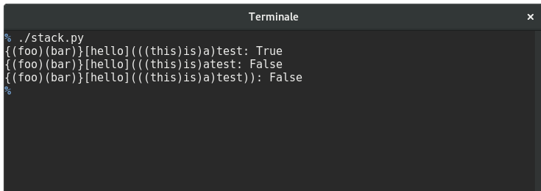
True, False, False. The code works. In summary, the push and pop operations of the stack data structure attract a O(1). The stack data structure is simply enough but is used to implement a whole range of functionality in the real world. The back and forward buttons on the browser are made possible by stacks. To be able to have undo and redo functionality in word processors, stacks are also used.
Queue
A special type of list is the queue data structure
- This data structure is no different from the regular queue you are accustomed to in real life. If you have stood in line at an airport or to be served your favorite burger at your neighborhood shop, then you should know how things work in a queue.Queues are also a very fundamental and important concept to grasp since many other data structures are built on them. The way a queue works is that the first person to join the queue usually gets served first, all things being equal. The acronym FIFO best explains this. FIFO stands for first in, first out. When people are standing in a queue waiting for their turn to be served, service is only rendered at the front of the queue. The only time people exit the queue is when they have been served, which only occurs at the very front of the queue. By strict definition, it is illegal for people to join the queue at the front where people are being served:
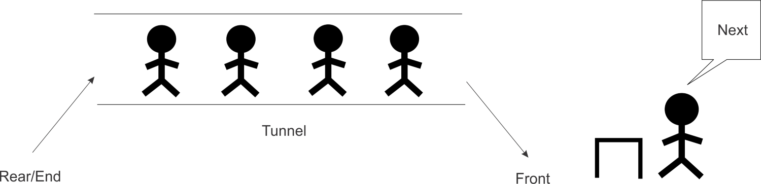
To join the queue, participants must first move behind the last person in the queue. The length of the queue does not matter. This is the only legal or permitted way by which the queue accepts new entrants.
As human as we are, the queues that we form do not conform to strict rules. It may have people who are already in the queue deciding to fall out or even have others substituting for them. It is not our intent to model all the dynamics that happen in a real queue. Abstracting what a queue is and how it behaves enables us to solve a plethora of challenges, especially in computing.
We shall provide various implementations of a queue but all will revolve around the same idea of FIFO. We shall call the operation to add an element to the queue enqueue. To remove an element from the queue, we will create a dequeue operation. Anytime an element is enqueued, the length or size of the queue increases by one. Conversely, dequeuing items reduce the number of elements in the queue by one.
To demonstrate the two operations, the following table shows the effect of adding and removing elements from a queue:
| Queue Operation | Size | Contents | Operatn results |
|---|---|---|---|
| Queue() | 0 | [] | Queue object created |
| Enqueue "Mark" | 1 | ['mark'] | Mark added to queue |
| Enqueue "John" | 2 | ['mark','john'] | John added to queue |
| Size() | 2 | ['mark','john'] | Number of items in queue returned |
| Dequeue() | 1 | ['mark'] | John is dequeued and returned |
| Dequeue() | 0 | [] | Mark is dequeued and returned |
Visualizing a Queue is easiest if you think of waiting in line at the bank with a “head” and “tail” on the line. Usually there’s a rope maze that has an entrance at the end and an exit where the tellers are located. You enter the queue by entering the “tail” of this rope maze line, and we’ll call that shift because that’s a common programming word in the Queue data structure. Once you enter the bank line (queue), you can’t just jump the line and leave or else people will get mad. So you wait, and as each person in front of you exits the line you get closer to exiting from the “head.” Once you reach the end then you can exit, and we’ll call that unshift. A Queue is therefore similar to a DoubleLinkedList because you are working from both ends of the data structure.
Note: Many times you can find real-world examples of a data structure to help you visualize how it works. You should take the time now to draw these scenarios or actually get a stack of books and test out the operations. How many other real situations can you find that are similar to a Stack and a Queue?
Queues
If we need more control over communication between processes, we can use a Queue. Queue data structures are useful for sending messages from one process into one or more other processes. Any picklable object can be sent into a Queue, but remember that pickling can be a costly operation, so keep such objects small. To illustrate queues, let's build a little search engine for text content that stores all relevant entries in memory.
This is not the most sensible way to build a text-based search engine, but I have used this pattern to query numerical data that needed to use CPU-intensive processes to construct a chart that was then rendered to the user.
This particular search engine scans all files in the current directory in parallel. A process is constructed for each core on the CPU. Each of these is instructed to load some of the files into memory. Let's look at the function that does the loading and searching:
def search(paths, query_q, results_q):
lines = []
for path in paths:
lines.extend(1.strip() for 1 in path.open())
query = query_q.get()
while query:
results_q.put([1 for 1 in lines if query in 1])
query = query_q.get()
Remember, this function is run in a different process (in fact, it is run in cpucount() different processes) from the main thread. It passes a list of path.path objects, and two multiprocessing.Queue objects; one for incoming queries and one to send outgoing results. These queues automatically pickle the data in the queue and pass it into the subprocess over a pipe. These two queues are set up in the main process and passed through the pipes into the search function inside the child processes.
The search code is pretty dumb, both in terms of efficiency and of capabilities; it loops over every line stored in memory and puts the matching ones in a list. The list is placed in a queue and passed back to the main process.
Let's look at the main process, which sets up these queues:
if _name_ == '_main_':
from multiprocessing import Process, Queue, cpu_count
from path import path
cpus = cpu_count()
pathnames = [f for f in path('.').listdir() if f.isfile()]
paths = [pathnames[i::cpus] for i in range(cpus)]
query_queues = [Queue() for p in range(cpus)]
results_queue = Queue()
search_procs = [
Process(target=search, args=(p, q, results_queue)
for p, q in zip(paths, query_queues)
]
for proc in search_procs: proc.start()
For an easier description, let's assume cpu_count is four. Notice how the import statements are placed inside the if guard? This is a small optimization that prevents them from being imported in each subprocess (where they aren't needed) on some operating systems. We list all the paths in the current directory and then split the list into four approximately equal parts. We also construct a list of four Queue objects to send data into each subprocess. Finally, we construct a single results queue. This is passed into all four of the subprocesses. Each of them can put data into the queue and it will be aggregated in the main process.
Now let's look at the code that makes a search actually happen:
for q in query_queues:
q.put("def")
q.put(None) # Signal process termination
for i in range(cpus):
for match in results_queue.get():
print(match)
for proc in search_procs:
proc.join()
This code performs a single search for "def" (because it's a common phrase in a directory full of Python files!).
This use of queues is actually a local version of what could become a distributed system. Imagine if the searches were being sent out to multiple computers and then recombined. Now imagine you had access to the millions of computers in Google's data centers and you might understand why they can return search results so quickly!
We won't discuss it here, but the multiprocessing module includes a manager class that can take a lot of the boilerplate out of the preceding code. There is even a version of multiprocessing.Manager that can manage subprocesses on remote systems to construct a rudimentary distributed application. Check the Python multiprocessing documentation if you are interested in pursuing this further.
FIFO Queue
The python Queue class implements a basic first-in, first-out collection. Items can be added to the end of the container using put(), and removed from the head using get().
The constructor for a FIFO queue is as follows:
class Queue.Queue(maxsize = 0)
The parameter maxsize is an integer used to limit the items that can be added into the queue.
Insertion will be blocked once the queue is full, until items are consumed. The queue size is infinite if maxsize <= 0.
See the following example for how to use the FIFO queue:
import Queue
q = Queue.Queue()
# put items at the end of the queue
for x in range(4):
q.put("item-" + str(x))
# remove items from the head of the queue
while not q.empty():
print q.get()
# the output
item-0
item-1
item-2
item-3
Creating a FIFO Queue
// Initialize queue
Syntax: queue.Queue(maxsize)
// Insert Element
Syntax: Queue.put(data)
// Get And remove the element
Syntax: Queue.get()
import queue
# From class queue, Queue is created as an object
# Now L is Queue of a maximum capacity of 20
L = queue.Queue(maxsize = 20)
# Data is inserted into Queue using put()
# Data is inserted at the end
L.put(5)
L.put(9)
L.put(1)
L.put(7)
# get() takes data out from the Queue from the head of the Queue
print(L.get())
print(L.get())
print(L.get())
print(L.get())
Output:
5
9
1
7
CASE STUDY: SIMULATING A SUPERMARKET CHECKOUT LINE
In this case study, you develop a program to simulate supermarket checkout stations. To keep the program simple, some important factors found in a realistic supermarket situation have been omitted; you’re asked to add them back as part of the exercises.
Request
Write a program that allows the user to predict the behavior of a supermarket checkout line under various conditions.
Analysis
For the sake of simplicity, the following restrictions are imposed:
Image There is just one checkout line, staffed by one cashier.
Image Each customer has the same number of items to check out and requires the same processing time.
Image The probability that a new customer will arrive at the checkout does not vary over time.
The inputs to the simulation program are the following:
Image The total time, in abstract minutes, that the simulation is supposed to run.
Image The number of minutes required to serve an individual customer.
Image The probability that a new customer will arrive at the checkout line during the next minute. This probability should be a floating-point number greater than 0 and less than or equal to 1.
The program’s outputs are the total number of customers processed, the number of customers left in the line when the time runs out, and the average waiting time for a customer. Table 8.3 summarizes the inputs and outputs.
| Inputs | Range of Value for Inputs | Outputs |
|---|---|---|
| Total minutes | 0<=total <= 1000 | Total customers processed |
| Average minutes per customer | 0<average <= total | Customers left in line |
| Probability of a new arrival in the next minute | 0<probability <= 1 | Average waiting time |
The User InterfaceThe following user interface for the system has been proposed:
Welcome the Market Simulator
Enter the total running time: 60
Enter the average time per customer: 3
Enter the probability of a new arrival: 0.25
TOTALS FOR THE CASHIER
Number of customers served: 16
Number of customers left in queue: 1
Average time customers spend
Waiting to be served: 2.38
Classes and Responsibilities
As far as classes and their overall responsibilities are concerned, the system is divided into a main function and several model classes. The main function is responsible for interacting with the user, validating the three input values, and communicating with the model. The design and implementation of this function require no comment, and the function’s code is not presented. The classes in the model are listed in the following table:
| Class | Responsibilities |
|---|---|
| MarketModel | A market model does the following: |
| 1. Runs the simulation | |
| 2. Creates a cashier object | |
| 3. Sends new customer objects to the cashier | |
| 4. Maintains an abstract clock | |
| 5. During each tick of the clock, tells the cashier to provide another unit of servie to a customer | |
| Cashier | A cashier object does the following: |
| 1. Contains a queue of customers objects | |
| 2. Adds new customer objects to this queue when directed to do so | |
| 3. Removes customers from the queue in turn | |
| 4. Gives the current customer a unit of service when directed to do so and releases the customer when the service has been completed | |
| Customer | A customer object: |
| 1. Knows its arrival time and how much service it needs | |
| 2. Knows when the cashier has provided enough service. The class as a whole generates new customers when directed to do so according to the probability of a new customer arriving | |
| LinkedQueue | Used by a cashier to represent a line of customers |
The relationships among these classes are shown in

The overall design of the system is reflected in the collaboration diagram shown

You can now design and implement each class in turn.
Because the checkout situation has been restricted, the design of the class MarketModel is fairly simple. The constructor does the following:
- Saves the inputs—probability of new arrival, length of simulation, and average time per customer.
- Creates the single cashier.
The only other method needed is runSimulation. This method runs the abstract clock that drives the checkout process. On each tick of the clock, the method does three things:
- Asks the Customer class to generate a new customer, which it may or may not do, depending on the probability of a new arrival and the output of a random number generator.
- If a new customer is generated, sends the new customer to the cashier.
- Tells the cashier to provide a unit of service to the current customer.
When the simulation ends, the runSimulation method returns the cashier’s results to the view. Here is the pseudocode for the method:
for each minute of the simulation
ask the Customer class to generate a new customer
if a customer is generated
cashier.addCustomer(customer)
cashier.serveCustomers(current time)
return cashier's results
Note: The pseudocode algorithm asks the Customer class for an instance of itself. Because it is only probable that a customer will arrive at any given minute, occasionally a customer will not be generated. Rather than code the logic for making this choice at this level, you can bury it in a class method in the Customer class. From the model, the Customer class method generateCustomer receives the probability of a new customer arriving, the current time, and the average time needed per customer. The method uses this information to determine whether to create a customer and, if it does, how to initialize the customer. The method returns either the new Customer object or the value None. The syntax of running a class method is just like that of an instance method, except that the name to the left of the dot is the class’s name.
Complete listing of the class MarketModel:
"""
File: marketmodel.py
"""
from cashier import Cashier
from customer import Customer
class MarketMode(object):
def _init_(self, lengthOfSimulation, averageTimePerCus, probabilityOfNewArrival):
self._probabilityOfNewArrival =\ probabilityOfNewArrival
self._lengthOfSimulation = lengthOfSimulation
self._averageTimePerCus = averageTimePerCus
self._cashier = Cashier()
def ruSimulation(self):
"""Run the clock for n ticks."""
for currentTime in range(self._lengthOfSimulation):
# Attemt to generate a new customer
customer = Customer.generateCustomer(self._probabilityOfNewArrival, currentTime, self._averageTimePerCus)
#send customer to cashier if successfully generated
if customer != None
self._cashier to provide another unit of service self._cashier.serveCustomers(currentTime)
def _str_(self):
return str(self._cashier)
A cashier is responsible for serving a queue of customers. During this process, the cashier tallies the customers served and the minutes they spend waiting in line. At the end of the simulation, the class’s str method returns these totals as well as the number of customers remaining in the queue. The class has the following instance variables:
totalCustomerWaitTime
customerServed
queue
currentCustomer
The last variable holds the customer currently being processed.
To allow the market model to send a new customer to a cashier, the class implements the method addCustomer. This method expects a customer as a parameter and adds the customer to the cashier’s queue.
The method serveCustomers handles the cashier’s activity during one clock tick. The method expects the current time as a parameter and responds in one of several different ways, as listed in
| Condition | What It Means | Action to Perform |
|---|---|---|
| The current customer is None and the queue is empty | There are no customers to serve | Noen;just return |
| The current customer is None and the queue is empty | There is a customer waiting at the front of the queue | 1. Pop a customer and make it the current customer |
| 2. Ask it when it was instantiated, determine how long it has been waiting, and add that time to the total waiting time for all customers | ||
| 3. Increment the number of customers served | ||
| 4. Give the customer a unit of service and dismiss it if it is finished | ||
| The current customer is not None | Serve the current customer | Give the customer one unit of service and dismiss it if it is finished |
Pseudocode for the method serveCustomers:
if currentCustomer is None:
if queue is empty:
return
else:
currentCustomer = queue.pop()
totalCustomerWaitTime = totalCustomerWaitTime + currentTime - currentCustomer.arrivalTime()
increment customerServed
currentCustomer.serve()
if currentCustomer.amountOfSeriveNeeded() == 0:
currentCustomer = None
Code for the Cashier class:
"""
File: cashier.py
"""
from linkedqueue import LinkedQueue
class Cashier(object):
def _init_(self):
self._totalCustomerWaitTime = 0
self._customersServed = 0
self._currentCustomer = None
self._queue = LinkedQueue()
def addCustomer(self, c):
self._queue.add(c)
def serveCustomers(self, currentTime):
if self._currentCustomer is None:
# No Customers yet
if self._queue.isEmpty():
return
else:
# Pop first waiting customer and tally results
self._currentCustomer = self._queue.pop()
self._totalCustomerWaitingTime += \ currentTime - \
self._currentCustomer.arrivalTime()
self._customersServed += 1
# Give a unit of service
self._currentCustomer.serve()
# If current customer is finished, send it away
if self._currentCustomer.amountOfServiceNeeded() == \
0:
self._currentCustomer = None
def _str_(self):
result = "TOTALS FOR THE CASHIER\n" + \
"Number of customers served: " +\
str(self._customersServed) + "\n"
if self._customersServed != 0:
aveWaitTime = self._totalCustomerWaitTime /\
self._customersServed
result += "Number of customers left in queue: " \
+ str(len(self._queue)) + "\n" + \
"Average time customers spend\n" + \
"watiting to be served: " \
+ "%5.2f" % aveWaitTime
return result
The Customer class maintains a customer’s arrival time and the amount of service needed. The constructor initializes these with data provided by the market model. The instance methods include the following:
Image arrivalTime()—Returns the time at which the customer arrived at a cashier’s queue.
Image amountOfServiceNeeded()—Returns the number of service units left.
Image serve()—Decrements the number of service units by one.
The remaining method, generateCustomer, is a class method. It expects as arguments the probability of a new customer arriving, the current time, and the number of service units per customer. The method returns a new instance of Customer with the given time and service units, provided the probability is greater than or equal to a random number between 0 and 1. Otherwise, the method returns None, indicating that no customer was generated. The syntax for defining a class method in Python is the following:
@classmethod
def <method name> (cls, <other parameters>):
<statement>
Code for the Customer class:
"""
File: customer.py
"""
import random
class Customer(object):
@classmethod
def generateCustomer(cls, probabilityOfNewArrival, arrivalTime, averageTimePerCustomer):
"""Returns a Customer ofject if the probability of arrival is greater than or equal to a random number.
otherwise, returns None, indicating no new customer."""
if random.random() <= probabilityOfNewArrival:
return Customer(arrivalTime, averageTimePerCustomer)
else:
return None
def _init_((self, arrivalTime, serviceNeeded):
self._arrivalTime = arrivalTime
self._amountOfServiceNeeded = serviceNeeded
def arrivalTime(self):
return self._arrivalTime
def amountOfServicNeeded (self):
return self._arrivalTime
def amountOfServiceNeeded(self):
return self._amountOfServiceNeeded
def serve(self):
"""Accepts a unit of service from the cashier."""
self._amountOfServiceNeeded -= 1
CASE STUDY: AN EMERGENCY ROOM SCHEDULER
As anyone who has been to a busy hospital emergency room knows, people must wait for service. Although everyone might appear to be waiting in the same place, they are actually in separate groups and scheduled according to the seriousness of their condition. This case study develops a program that performs this scheduling with a priority queue.
Request
Write a program that allows a supervisor to schedule treatments for patients coming into a hospital’s emergency room. Assume that, because some patients are in more critical condition than others, patients are not treated on a strictly first-come, first-served basis, but are assigned a priority when admitted. Patients with a high priority receive attention before those with a lower priority.
Analysis
Patients come into the emergency room in one of three conditions. In order of priority, the conditions are ranked as follows:
- Critical
- Serious
- Fair
When the user selects the Schedule option, the program allows the user to enter a patient’s name and condition, and the patient is placed in line for treatment according to the severity of his condition. When the user selects the Treat Next Patient option, the program removes and displays the patient first in line with the most serious condition. When the user selects the Treat All Patients option, the program removes and displays all patients in order from patient to serve first to patient to serve last.
Each command button produces an appropriate message in the output area. This Table lists the interface’s responses to the commands.
| User Command | Program Response |
|---|---|
| Schedule | Prompts the user for the patient's name and condition, and then prints {patient name} is added to the {condition} list |
| Treat Next Patient | Prints{patient name} is being treated |
| Treat All Patients | Prints{patient name} is being treated....Prints {patent name} is being treated |
Here is an interaction with the terminal-based interface:
Main Menu
1 Schedule a patient
2 Treat the next patient
3 Treat all patients
4 Exit the program
Enter a number [1-4]: 1
Enter the patient's name: Larry
Patient's condition:
1 Critical
2 Serious
3 Fair
Enter a number [1-3]: 1
Larry is added to the critical list.
Main menu
1 Schedule a patient
2 Treat the next patient
3 Treat all patients
4 Exit the program
Enter a number [1-4]: 3
Larry/ critical is being treated.
Steve/ serious is being treated.
Laura/ fair is being treated.
No patients available to treat.
Classes The application consists of a view class, called ERView, and a set of model classes. The view class interacts with the user and runs methods with the model. The class ERModel maintains a priority queue of patients. The class Patient represents patients, and the class Condition represents the three possible conditions. The relationships among the classes are shown in the next Figure
Design and Implementation
The Patient and Condition classes maintain a patient’s name and condition. You can compare (according to their conditions) and view them as strings. Here is the code for these two classes:
class Condition(object):
def _init_(self, rank):
self._rank = rank
def _ge_(self, other):
"""Used for comparison,"""
return self._rank >= other._rank
def _str_(self):
if self._rank == 1: return "critical"
elif self._rank == 2: return "serious"
else: return "fair"
class Patient(object)
def _init_(self, name, condition):
self._name = name
self._condition = condition
def _ge_(self, other):
"""Used for comparisons."""
return self._conditions >= other._conditions
def _str_(self):
return self._name + " /" + str(self._condition)
The class ERView uses a typical menu-driven loop. You structure the code using several helper methods. Here is a complete listing:
"""
File: erapp.py
The view for an emergency room scheduler.
"""
from model import ERModel, Patient, Condition
class ERView(object):
""" The view class for the ER application"""
def _init_(self, model):
self._model = model
def run(self):
"""Menu-driven comand loop for the app."""
menu = "Main menu\n" + \
" 1 Schedule a patient\n" + \
" 2 Treat the next patient\n" + \
" 3 Treat all patients\n" \
" 4 Exit the program\n"
while True:
command = self._getCommand(4, menu)
if command == 1: self._schedule()
elif command == 2: self._treatNext()
elif command == 3: self._treatAll()
else: break
def treatNext(self):
"""Treats one patient if there is one."""
if self.model.isEmpty():
print("No patients available to treat")
else:
patient = self.model.treatNext()
print(patient, "is being treated.")
def treatAll(self):
""" Treats all the remaining patients."""
if self.model.isEmpty():
print("No patients available to treat.")
else:
while not self.model.isEmpty():
self.treatNext()
def _schedule(self):
"""Obtains patient info and schedules patient."""
name = input("\nEnter the patient's name: ")
condition = self._getCondition()
self._model.schedule(Patient(name, condition))
print(name, "is added to the", condition, "list\n")
def _getCondition(self):
"""Obtains condition info."""
menu = "Patient's condition:\n" + \
" 1 Critical\n" + \
" 2 Serious\n" + \
" 3 Fair\n"
number = self._getCommand(3, menu)
return Condition(number)
def_getCommand(self._getCommand(3, menu)
"""Obtains and returns a command number."""
prompt = "Enter a number [1-" + str(high) + "]: "
commandRange = list(map(str, range(1, high + 1)))
error = "Error, number must be 1 to " + str(high)
while True:
print (menu)
command = input(prompt)
if command in comandRange:
return int(command)
else:
print(error)
# Main function to start up the application
def main():
model = ERModel()
view = ERView(model)
view.run()
if _name_ == "_main_":
main()
The class ERModel uses a priority queue to schedule the patients. Its implementation is left as a programming project for you.
STUDENT PERFORMANCE LAB
- Complete the emergency room scheduler application as described in the case study.
Checkout Performance Lab Exercises:
In real life, customers do not choose a random cashier when they check out. They typically base their choice on at least the following two factors:
- The length of a line of customers waiting to check out.
- The physical proximity of a cashier.
Modify the simulation of the previous project exercise so that it takes account of the first factor.
Modify the simulation of the previous project so that it takes account of both factors listed in that project. You should assume that a customer initially arrives at the checkout line of a random cashier and then chooses a cashier who is no more than two lines away from this spot. This simulation should have at least four cashiers.
The simulator’s interface asks the user to enter the average number of minutes required to process a customer. However, as written, the simulation assigns the same processing time to each customer. In real life, processing times vary around the average. Modify the Customer class’s constructor so it randomly generates service times between 1 and (average * 2 + 1).
Please submit your work prior to continuing
General Trees
Thinking Nonlinearly
In this topic, we will discuss one of the most important nonlinear data structures in computing—trees. Tree structures are indeed a breakthrough in data organization, for they allow us to implement a host of algorithms much faster than when using linear data structures, such as array-based lists or linked lists. Additionally, trees provide a natural organization for data, and consequently have become ubiquitous structures in file systems, graphical user interfaces, databases, Web sites, and other computer systems.
It is not always clear what productivity experts mean by “nonlinear” thinking, but when we say that trees are “nonlinear,” we are referring to an organizational relationship that is richer than the simple “before” and “after” relationships between objects in sequences. The relationships in a tree are hierarchical, with some objects being “above” and some “below” others. Actually, the main terminology for tree data structures comes from family trees, with the terms “parent,” “child,” “ancestor,” and “descendant” being the most common words used to describe relationships.
EFamily Tree

TREE DEFINITIONS AND PROPERTIES
A tree is an abstract data type that stores elements hierarchically. With the exception of the top element, each element in a tree has a parent element and zero or more children elements. A tree is usually visualized by placing elements inside ovals or rectangles, and by drawing the connections between parents and children with straight lines. (See Figure below) We typically call the top element the root of the tree, but it is drawn as the highest element, with the other elements being connected below (just the opposite of a botanical tree).
A tree with 17 nodes representing the organization of a fictitious corporation. The root stores Electronics R'Us. The children of the root store R & D, Sales, Purchasing, and Manufacturing. The internal nodes store Sales, International, Overseas, Electronics R'Us, and Manufacturing.
Formal Tree Definition
Formally, we define a tree T as a set of nodes storing elements such that the nodes have a parent-child relationship that satisfies the following properties:
If T is nonempty, it has a special node, called the root of T, that has no parent. Each node v of T different from the root has a unique parent node w; every node with parent w is a child of w. Note that according to our definition, a tree can be empty, meaning that it does not have any nodes. This convention also allows us to define a tree recursively such that a tree T is either empty or consists of a node r, called the root of T, and a (possibly empty) set of subtrees whose roots are the children of r.
Other Node Relationships
Two nodes that are children of the same parent are siblings. A node v is external if v has no children. A node v is internal if it has one or more children. External nodes are also known as leaves.
Example:
Earlier, we discussed the hierarchical relationship between files and directories in a computer's ile system, although at the time we did not emphasize the nomenclature of a ile system as a tree. In Figure below, we revisit an earlier example. We see that the internal nodes of the tree are associated with directories and the leaves are associated with regular iles. In the UNIX and Linux operating systems, the root of the tree is appropriately called the “root directory” and is represented by the symbol “/.”
Tree Representation of a File System
A node u is an ancestor of a node v if u = v or u is an ancestor of the parent of v. Conversely, we say that a node v is a descendant of a node u if u is an ancestor of v. For example, in Figure above, cs252/ is an ancestor of papers/, and pr3 is a descendant of cs016/. The subtree of T rooted at a node v is the tree consisting of all the descendants of v in T (including v itself). In Figure above, the subtree rooted at cs016/ consists of the nodes cs016/, grades, homeworks/, programs/, hw1, hw2, hw3, pr1, pr2, and pr3.
Edges and Paths in Trees
An edge of tree T is a pair of nodes (u, v) such that u is the parent of v, or vice versa. A path of T is a sequence of nodes such that any two consecutive nodes in the sequence form an edge. For example, the tree in Figure 8.3 contains the path (cs252/, projects/, demos/, market).
Example: The inheritance relation between classes in a Python program forms a tree when single inheritance is used. For example, in Section 2.4 we provided a summary of the hierarchy for Python's exception types, as portrayed in Figure below.
The BaseException class is the root of that hierarchy, while all user-defined exception classes should conventionally be declared as descendants of the more specific Exception class.
Python's hierarchy of Exception Types
In Python, all classes are organized into a single hierarchy, as there exists a built-in class named object as the ultimate base class. It is a direct or indirect base class of all other types in Python (even if not declared as such when defining a new class). Therefore, the hierarchy pictured in Figure above is only a portion of Python's complete class hierarchy.
Building trees
The process of assembling a tree is similar to the process of assembling a linked list. Each constructor invocation builds a single node.
class Tree:
def _init_(self, cargo, left=None, right=None):
self.cargo = cargo
self.left = left
self.right = right
def _str_(self):
return str(self.cargo)
The cargo can be any type, but the left and right parameters should be tree nodes. left and right are optional; the default value is None.
To print a node, we just print the cargo.
One way to build a tree is from the bottom up. Allocate the child nodes first:
left = Tree(2)
right = Tree(3)
Then create the parent node and link it to the children:
tree = Tree(1, left, right);
We can write this code more concisely by nesting constructor invocations:
>>> tree = Tree(1, Tree(2), Tree(3))
Either way, the result is the tree at the beginning.
Traversing trees Any time you see a new data structure, your first question should be, How do I traverse it? The most natural way to traverse a tree is recursively. For example, if the tree contains integers as cargo, this function returns their sum:
def total(tree):
if tree == None: return 0
return total(tree.left) + total(tree.right) + tree.cargo
The base case is the empty tree, which contains no cargo, so the sum is 0. The recursive step makes two recursive calls to find the sum of the child trees. When the recursive calls complete, we add the cargo of the parent and return the total.
Expression trees A tree is a natural way to represent the structure of an expression. Unlike other notations, it can represent the computation unambiguously. For example, the infix expression 1 + 2 * 3 is ambiguous unless we know that the multiplication happens before the addition.
This expression tree represents the same computation:
The nodes of an expression tree can be operands like 1 and 2 or operators like + and *. Operands are leaf nodes; operator nodes contain references to their operands. (All of these operators are binary, meaning they have exactly two operands.)
We can build this tree like this:
>>> tree = Tree('+', Tree(1), Tree('*', Tree(2), Tree(3)))
Looking at the figure, there is no question what the order of operations is; the multiplication happens first in order to compute the second operand of the addition.
Expression trees have many uses. The example in this chapter uses trees to translate expressions to postfix, prefix, and infix. Similar trees are used inside compilers to parse, optimize, and translate programs.
Tree traversal We can traverse an expression tree and print the contents like this:
def print_tree(tree):
if tree == None: return
print tree.cargo,
print_tree(tree.left)
print_tree(tree.right)
In other words, to print a tree, first print the contents of the root, then print the entire left subtree, and then print the entire right subtree. This way of traversing a tree is called a preorder, because the contents of the root appear before the contents of the children. For the previous example, the output is:
>>> tree = Tree('+', Tree(1), Tree('*', Tree(2), Tree(3)))
>>> print_tree(tree)
+ 1 * 2 3
This format is different from both postfix and infix; it is another notation called prefix, in which the operators appear before their operands.
You might suspect that if you traverse the tree in a different order, you will get the expression in a different notation. For example, if you print the subtrees first and then the root node, you get:
def print_tree_postorder(tree):
if tree == None: return
print_tree_postorder(tree.left)
print_tree_postorder(tree.right)
print tree.cargo,
The result, 1 2 3 * +, is in postfix! This order of traversal is called postorder.
Finally, to traverse a tree inorder, you print the left tree, then the root, and then the right tree:
def print_tree_inorder(tree):
if tree == None: return
print_tree_inorder(tree.left)
print tree.cargo,
print_tree_inorder(tree.right)
The result is 1 + 2 * 3, which is the expression in infix.
To be fair, we should point out that we have omitted an important complication. Sometimes when we write an expression in infix, we have to use parentheses to preserve the order of operations. So an inorder traversal is not quite sufficient to generate an infix expression.
Nevertheless, with a few improvements, the expression tree and the three recursive traversals provide a general way to translate expressions from one format to another.
If we do an inorder traversal and keep track of what level in the tree we are on, we can generate a graphical representation of a tree:
def print_tree_indented(tree, level=0):
if tree == None: return
print_tree_indented(tree.right, level+1)
print ' ' * level + str(tree.cargo)
print_tree_indented(tree.left, level+1)
The parameter level keeps track of where we are in the tree. By default, it is initially 0. Each time we make a recursive call, we pass level+1 because the child’s level is always one greater than the parent’s. Each item is indented by two spaces per level. The result for the example tree is:
>>> print_tree_indented(tree)
3
*
2
+
1
If you look at the output sideways, you see a simplified version of the original figure.
Python Binary Search
Python Program for First Binary Tree Search - implementing Recursion
This is a Python program to perform depth-first search on a binary tree using recursion. Problem Description The program creates a binary tree and presents a menu to the user to perform operations on the tree including depth-first search. Problem Solution
1. Create a class BinaryTree with instance variables key, left and right.
2. Define methods set_root, insert_left, insert_right, depth_first and search.
3. The method set_root takes a key as argument and sets the variable key equal to it.
4. The methods insert_left and insert_right insert a node as the left and right child respectively.
5. The method depth_first displays a depth first traversal of the tree.
6. The method search returns a node with a specified key.
Python Program for First Binary Tree Search - without using Recursion
This is a Python program to perform depth-first search on a binary tree without using recursion. Problem Description The program creates a binary tree and presents a menu to the user to perform operations on the tree including depth-first search. Problem Solution
1. Create a class Stack to implement a stack.
2. The class Stack will have methods is_empty, push and pop.
3. Create a class BinaryTree with instance variables key, left and right.
4. Define methods set_root, insert_left, insert_right, preorder_depth_first and search.
5. The method set_root takes a key as argument and sets the variable key equal to it.
6. The methods insert_left and insert_right insert a node as the left and right child respectively.
7. The method search returns a node with a specified key.
8. The method preorder_depth_first displays a preorder DFS traversal of the tree.
9. The preorder traversal is implemented using a stack to avoid recursion.
Python Program to Find Nth Node in the Inorder Traversal of a Binary Tree
This is a Python program to find the Nth node in the in-order traversal of a binary tree. Problem Description The program creates a binary tree and presents a menu to the user to perform operations on the tree including printing the Nth term in its in-order traversal. Problem Solution
1. Create a class BinaryTree with instance variables key, left and right.
2. Define methods set_root, insert_left, insert_right, inorder_nth, inorder_nth_helper and search.
3. The method set_root takes a key as argument and sets the variable key equal to it.
4. The methods insert_left and insert_right insert a node as the left and right child respectively.
5. The method search returns a node with a specified key.
6. The method inorder_nth displays the nth element in the in-order traversal of the tree. It calls the recursive method inorder_nth_helper.
Performance Lab Set #1
Task 1
- Use the following Tree to answer the six questions.
- What are the leaf nodes in the tree?
- What are the interior nodes in the tree?
- What are the siblings of node 7?
- What is the height of the tree?
- How many nodes are in level 2?
- Is the tree a general tree, a binary tree, or both?
Task 2
- What is the difference between a perfectly balanced binary tree and a complete binary tree?
- What is the difference between a complete binary tree and a full binary tree?
- A full binary tree has a height of 5. How many nodes does it contain?
- A complete binary tree contains 125 nodes. What is its height?
- How many nodes are on a given level L in a full binary tree? Express your answer in terms ofL.
Task 3
- What is the heap property for a min-heap?
- How is a binary search tree different from a binary tree?
- Write the expression represented by the following expression tree in infix, prefix, and postfix notations.(Hint: Use the inorder, preorder, and postorder traversals described in this section to obtain your answers.)
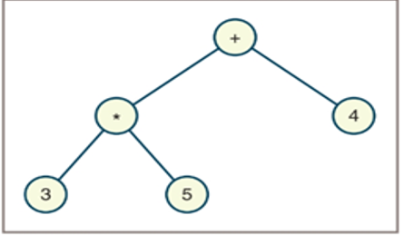
- Draw diagrams of the expression trees for the following expressions: a. 35 + 6 b. 3 + 56 c. 356
Task 4
- Describe how insertions can have a negative effect on subsequent searches of a binary search tree.
- Discuss the trade-offs between the array-based implementation of a sorted bag presented in Chapter 6 and a binary search tree implementation of a sorted bag.
Task 5
- Assume that a node is at position 12 in an array representation of a binary tree. Give the positions of that node's parent, left child, and right child.
- Whar are the constraints on a binary tree that is contained in an array?
Task 6
- How do the run times of the heap operation differ from their counterparts in binary search trees?
- What is the advantage of using a list over using an array to implement a heap?
- The heap sort uses a heap to sort a list of items. The strategy of this sort is to add the items in the list to a heap and then remove all of them from the heap as they are transferred back to the list. What is the run time and memory complexity of the heap sort?
Performance Lab Set #2
- Write a Python program to create a Balanced Binary Search Tree (BST) using an array (given) elements where array elements are sorted in ascending order.
- Write a Python program to find the closest value of a given target value in a given non-empty Binary Search Tree (BST) of unique values.
- Write a Python program to check whether a given a binary tree is a valid binary search tree (BST) or not.
Let a binary search tree (BST) is defined as follows: The left subtree of a node contains only nodes with keys less than the node's key. The right subtree of a node contains only nodes with keys greater than the node's key. Both the left and right subtrees must also be binary search trees.
Example 1:
2
/ \
1 3
Binary tree [2,1,3], return true.
Example 2:
1
/ \
2 3
Binary tree [1,2,3], return false.
-
Write a Python program to delete a node with the given key in a given Binary search tree (BST).
Note: Search for a node to remove. If the node is found, delete the node. -
Write a Python program to convert a given array elements to a height balanced Binary Search Tree (BST).
-
Write a Python program to find the kth smallest element in a given a binary search tree.
Submit your assignment
Advanced
Introduction:
This lesson you will quickly dive into more advanced uses and features of Python.
Topics Covered:
- CTypes and Structures
- Loading Libraries
- Structures
- Regular Expressions
- Additional Libraries and Modules
- Multithreading
- Unit Testing
- Metaclasses
To access the Advanced Python slides please click here
Objectives
CTypes and Structures
CTypes and Structures
CTypes provide C compatible data types and allow function calls from DLLs or shared libraries without having to write custom C extensions for every operation. So we can access the functionality of a C library from the safety and comfort of the Python Standard Library.
CTypes are a Foreign Function Interface (FFI) library and provide an API for creating C-compatible datatypes.
Reference: CTypes
Loading Libraries:
There are four types of dynamic library loaders available in ctypes and two conventions to use them. The classes that represent dynamic and shared libraries are ctypes.CDLL, ctypes.PyDLL, ctypes.OleDLL, and ctypes.WinDLL. The last two are only available on Windows.
Differences between CDLL and PyDLL:
ctypes.CDLL: This class represents loaded shared libraries. The functions in these libraries use the standard calling convention, and are assumed to returnint. GIL (Global Interpreter Lock) is released during the call. (More on GIL)ctypes.PyDLL: This class works likeCDLL, but GIL is not released during the call. After execution, the Python error flag is checked and an exception is raised if it is set. It is only useful when directly calling functions from the Python/C API.
To load a library, you can either instantiate one of the preceding classes with proper arguments or call the LoadLibrary() function from the submodule associated with a specific class:
ctypes.cdll.LoadLibrary()forctypes.CDLLctypes.pydll.LoadLibrary()forctypes.PyDLLctypes.windll.LoadLibrary()forctypes.WinDLLctypes.oledll.LoadLibrary()forctypes.OleDLL
The main challenge when loading shared libraries is how to find them in a portable way. Different systems use different suffixes for shared libraries (.dll on Windows, .dylib on OS X, .so on Linux) and search for them in different places. Unfortunately, Windows does not have a predefined naming scheme for libraries.
Reference: CType Shared Libraries in Windows
Both library loading conventions (the LoadLibrary() function and specific library-type classes) require you to use the full library name. This means all the predefined library prefixes and suffixes need to be included. For example, to load the C standard library on Linux, you need to write the following:
>>> import ctypes
>>> ctypes.cdll.LoadLibrary('libc.so.6')
<CDLL 'libc.so.6', handle 7f0603e5f000 at 7f0603d4cbd0>
Fortunately, the ctypes.util submodule provides a find_library() function that allows to load a library using its name without any prefixes or suffixes and will work on any system that has a predefined scheme for naming shared libraries:
>>> import ctypes
>>> from ctypes.util import find_library
>>> ctypes.cdll.LoadLibrary(find_library('c'))
<CDLL '/usr/lib/libc.dylib', handle 7fff69b97c98 at 0x101b73ac8>
>>> ctypes.cdll.LoadLibrary(find_library('bz2'))
<CDLL '/usr/lib/libbz2.dylib', handle 10042d170 at 0x101b6ee80>
>>> ctypes.cdll.LoadLibrary(find_library('AGL'))
<CDLL '/System/Library/Frameworks/AGL.framework/AGL', handle 101811610 at 0x101b73a58>
#Linux
Calling C functions using ctypes
When the library is successfully loaded, the common pattern is to store it as a module-level variable with the same name as library. The functions can be accessed as object attributes, so calling them is like calling a Python function from any other imported module:
>>> import ctypes
>>> from ctypes.util import find_library
>>>
>>> libc = ctypes.cdll.LoadLibrary(find_library('c'))
>>>
>>> libc.printf(b"Hello world!\n")
Hello world!
Unfortunately, all the built-in Python types except integers, strings, and bytes are incompatible with C datatypes and thus must be wrapped in the corresponding classes provided by the ctypes module.
Data Types

As you can see, this table does not contain dedicated types that would reflect any of the Python collections as C arrays. The recommended way to create types for C arrays is to simply use the multiplication operator with the desired basic ctypes type:
>>> import ctypes
>>> IntArray5 = ctypes.c_int * 5
>>> c_int_array = IntArray5(1, 2, 3, 4, 5)
>>> FloatArray2 = ctypes.c_float * 2
>>> c_float_array = FloatArray2(0, 3.14)
>>> c_float_array[1]
3.140000104904175
Defining Argument Types and Return Types
If a C library requires arguments to be passed and/or has a return value, it is a good practice to declare them like so:
import ctypes
calc = ctypes.CDLL("MyCalc.dll")
addition = calc.addition()
# Declare return type
addition.restype = ctypes.c_int
# Declare argument types
addition.argtypes = [ctypes.c_int, ctypes.c_int]
# Pass arguments
addition(1,2)
Structures
Creating C Structs in Python can be useful. For instance, let's assume a function within a DLL requires a pointer to a struct to be passed. A real world example of this would be a DLL file that communicates with hardware. Below is an example of how to create a C struct using Python ctypes
import ctypes
# Create the struct
class P_Struct(ctypes.Structure):
_fields_ = [("field_1", ctypes.c_int),
("field_2", ctypes.c_char_p)]
# Pass struct values
my_struct = P_Struct(1, "Hello World")
# Create a pointer to my_struct
pointer_my_struct = ctypes.pointer(my_struct)
print my_struct.field_1, my_struct.field_2
# Import the DLL and pass pointer_my_struct to the C function requiring a pointer to a struct.
Output:
1 Hello World
Regular Expressions
Regular expressions, often referred to as REs or regexes, are bits of small and highly specialized programming language embedded inside Python. The PyDocs actually contains an entire page on how to use regex. We will be touching on some of it's functionality... it'll be up to you to utilize the PyDocs and take your knowledge to the next level.
PyDocs HOWTO
https://docs.python.org/3/howto/regex.html
PyDocs Re
https://docs.python.org/2/library/re.html
Using Regular Expressions
re.compile: compiles regular expression into pattern objects which allows for repeated use
re.match: apply pattern to the start of a string, return match or None
re.search: scan through a string, return match or None
re.findall: find all matches and return them as a list
Python re search and compile example:
import re
search_str = "This is a string to search"
re_search = re.compile("string")
matched_obj = re_search.search(search_str)
print matched_obj
<_sre.SRE_Match object at 0x02CBFA68>
Practical Example
import re
patterns = ['Enterprise', 'Death Star']
pharse = "The Enterprise is the flagship of the Federation."
for pattern in patterns:
print 'Looking for "{}" in "{}": '.format(pattern, pharse)
if re.search(pattern, pharse):
print "found a match!"
else:
print "no match!"
Looking for "Enterprise" in "The Enterprise is the flagship of the Federation.":
found a match!
Looking for "Death Star" in "The Enterprise is the flagship of the Federation.":
no match!
Python re search start() and end():
import re
pattern = "Dave"
text = "I'm sorry Dave, I'm afarid I can't do that."
match = re.search(pattern, text)
start = match.start()
end = match.end()
print 'Found "{}" in "{}" from {} to {} ("{}")'.format(match.re.pattern, match.string, start, end, text[start:end])
Found "Dave" in "I'm sorry Dave, I'm afarid I can't do that." from 10 to 14 ("Dave")
Python re match example:
Python's re.match is similar to re.search. The main difference being that match searches only at the start of the string whereas search will apply the pattern to the entire string.
import re
text = "I turned myself into a pickle. I'm Pickle Riiiiick."
text2 = "I did not turn myself into a pickle. I am not Pickle Riiiiick."
match = re.match("I turned myself", text)
match2 = re.match("I did not", text2)
if match == None:
print 'Could not find "{}" in "{}"'.format(match.re.pattern, match.string)
else:
print 'Found "{}" in "{}"'.format(match.re.pattern, match.string)
if match2 == None:
print 'Cound not find "{}" in "{}"'.format(match2.re.pattern, match2.string)
else:
print 'Found "{}" in "{}"'.format(match2.re.pattern, match2.string)
Found "I turned myself" in "I turned myself into a pickle. I'm Pickle Riiiiick"
Found "I did not" in "I did not turn myself into a pickle. I am not Pickle Riiiiick."
Additional Libraries and Modules
A few:
- sys, os, socket, glob, subprocess, hashlib, shutil, math, json
- struct
- 3rd party
- Paramiko
- pip
- pickle
- Hitchhikers Guide
Sys, OS and Subprocess
- sys module
- Contains system level info
- sys.path, sys.argv, sys.modules
- os module
- interact with the os dependent functionality
- os.path, os.walk, os.system, os.stat
- subprocess module
- spawn process, stdin/stdout
- subprocess.Popen()
Hashlib
Hashlib implements a common interface to many different secure hash and message digest algorithms.
import hashlib
m = hashlib.md5()
m.update("password")
print m.digest()
print m.hexdigest()
x = hashlib.md5()
x.update("password")
print m.digest()
if m.digest() == x.digest():
print 'access granted'
Struct
Struct performs conversions between Python values and C structs represented as Python strings. This is mostly used in handling binary data in files and network connections. This will be used during Network Programming.
import struct
data = struct.pack('hh1', 1, 2)
print data
data = struct.unpack('hh1', data)
print data
JSON
JSON is a lightweight data interchange format inspired by JavaScript object literal syntax. JSON is used in a whole lot of applications and scenarios.
import json
# JSON to Python
json_string = '{"make": "Ford", "model": "Mustang"}'
parsed_json = json.loads(json_string)
print parsed_json['make']
# Python to JSON
json_d = {
'make': 'Ford',
'model': 'Mustang',
'type': 'Pony',
'colors': ['red', 'blue', 'white', 'yellow']
}
parsed_d = json.dumps(json_d)
print parsed_d
Paramiko, PIP and the HitchHiker's Guide
Paramiko
Paramiko is a Python (2.7, 3.4+) implementation of SSHv2 protocol. Paramiko utilizes a Python C extension for low level crytography; though Paramiko itself utilizes a Python interface around SSH network concepts.
PIP
pip is a tool for installing Python packages. There is all sorts of packages you can install from virtualenv (Python virtual environments), Requests (http library) to Scrapy (webscraping). Since you have Python already installed, you have pip. Below is an example on how to install virtualenv.
pip install virtualenv
Easy. Here is a great list of some of the most popular Python packages.
https://pythontips.com/2013/07/30/20-python-libraries-you-cant-live-without/
pickle
Pickling is Python's way of serializing data. When you serialize data you're converting your object into a stream of bytes that you can save to a file for later use. pickle is part of the Python standard library. In order to access the module you must import it.
import pickle
You can pickle or serialize objects with the pick module, and you can also do the reverse which is known as unpickling, or deserializing the object.
After you've imported the pickle module the typical process is as follows:
- Open a file for binary writing
- Call the dump method to pickle your object
- After pickling all objects you want, close the file
You can pickle just about any type of object including:
- lists, tuples, dictionaries, sets, strings, ints, and floats
In order to pickle an object we can use the following methods:
pickle.dump(object, file)
pickle.dumps(object)
The difference between dump() and dumps() is that the dump method will take an argument for a file you want to write your serialized object to, while the dumps method simply will return the pickled representation of the object as a bytes object. You can then later write it to a file if you so choose.
In order to unpickle our object we can use the following methods:
pickle.load(inputfile)
pickle.loads(data)
The difference between load() and loads() is that the load method will read the pickled representation of an object from the open file object, while the loads will return the representation of your data object.
NOTE: Remember that the pickle module is not secure. Only unpickle data that you trust. It is possible to construct malicious pickle data which will execute arbitrary code during unpickling
To learn more: pickle documentation
The HitchHiker's Guide
The HitchHiker's guide is an excellent guide on Python that is constantly being updated.
http://docs.python-guide.org/en/latest/
Multithreading

Multithreading is similar to running multiple programs concurrently... but better.
- Threads within a process share the same data space with the main thread.
- Requires less memory overhead and is cheaper than running multiple processes
A thread has a beginning, execution sequence and conclusion. An instruction pointer keeps track of where it is currently running.
- Threads can be put to sleep, even while other threads are running.
- Threads can also be pre-empted (interrupted)
Multithreading Example:
import time
from threading import Thread
# Work to be done
def sleeper(i):
print "thread {:d} sleeps for 5 seconds\n".format(i)
time.sleep(5)
print "thread {:d} woke up\n".format(i)
# Creating the workers, and passing individual arguments to each of them
for i in range(10):
t = Thread(target=sleeper, args=(i,))
t.start()
thread 0 sleeps for 5 seconds
thread 1 sleeps for 5 seconds
thread 2 sleeps for 5 seconds
thread 3 sleeps for 5 seconds
thread 4 sleeps for 5 seconds
thread 5 sleeps for 5 seconds
thread 6 sleeps for 5 seconds
thread 7 sleeps for 5 seconds
thread 8 sleeps for 5 seconds
thread 9 sleeps for 5 seconds
thread 9 woke up
thread 7 woke up
thread 6 woke up
thread 4 woke up
thread 2 woke up
thread 1 woke up
thread 8 woke up
thread 0 woke up
thread 5 woke up
thread 3 woke up
Your output may not look like mine... that is okay. The time in which the workers start is almost always random due to how concurrent their launch sequences are.
UnitTesting
UnitTesting
Unit testing is a development process where parts of small code (called units) are individually and independently tested for proper operation. This can of course be done manually... but it is more often automated. This is an extremely important habit to build.
Python offers a powerful built in unit testing module called unittest.
References: HitchHiker's Guide, PyDocs
Example:
import unittest
def addx(x):
return x + 1
class MyTest(unittest.TestCase):
def test(self):
# is addX(3) == 4?
self.assertEqual(addx(3), 4)
# Run test on file launch
if __name__ == '__main__':
unittest.main()
- Above, we define a function in which we want to test... a unit.
- Then we create a test class and make it a child of TestCase
- Then we call upon one of the many assert methods. (https://docs.python.org/2/library/unittest.html#assert-methods)
Output:
----------------------------------------------------------------------
Ran 1 test in 0.001s
OK
In our case, this is exactly what we want to see. But what happens if the test case fails? Let's pass in the argument 4 to addx and see.
F
======================================================================
FAIL: test (__main__.MyTest)
----------------------------------------------------------------------
Traceback (most recent call last):
File ".\unit_testing.py", line 9, in test
self.assertEqual(addx(4), 4)
AssertionError: 5 != 4
----------------------------------------------------------------------
Ran 1 test in 0.001s
FAILED (failures=1)
- We get a nice fat F for failure
- Where the file failed
- The normal traceback
- The AssertionError which breaks down a more readable reason why it failed
- The runtime for each test
- And a FAILED status indicating how many failures.
Doctest
The doctest module searches for sections of text that look like interactive Python sessions in docstrings, and then executes them to verify that they work.
def addition(x, y):
""" Return x plus y
>>> addition(3, 3)
6
>>> addition(5, 2)
1
"""
return x + y
if __name__ == '__main__':
import doctest
doctest.testmod()
**********************************************************************
File ".\unit_testing.py", line 6, in __main__.addition
Failed example:
addition(5, 2)
Expected:
1
Got:
7
**********************************************************************
1 items had failures:
1 of 2 in __main__.addition
***Test Failed*** 1 failures.
PS C:\Users\xconstaud\Documents\Python\re>
Conclusion
As you have guessed, this can be insanly useful. In most cases, spending the extra time unit testing will save you a lot more time over debugging.
Metaclasses

Defined as “the class of a class”.
- Any class whose instances are themselves classes.
- type is a metaclass for instance; it creates classes!
- Used to construct classes. (always happens under hood)
- Can create dynamic classes with less lines using type.
- Think: instances are to classes as classes are to metaclasses.
- To create a metaclass, create a class that inherits from type
# in the most simple form
class Meta(type):
pass
- Classes are normally created with the type metaclass
- We can create a class with a different metaclass:
# Python 2
class Final(object):
__metaclass__ = Meta
# Python 3
class Final(metaclass=Meta):
pass
__new__(): It’s a method which is called before __init__(). It creates the object and return it.
__init__(): This method just initialize the created object passed as parameter
Example:
class Meta(type):
def __init__(cls, name, bases, dct):
print "Creating class {} using Meta".format(name)
super(Meta, cls).__init__(name, bases, dct)
class Foo(object):
__metaclass__ = Meta
class FooBar(Foo):
pass
First we create a new metaclass called Meta:
- On the construction of classes built using Meta, we print out that we are creating a class using Meta.
Next, create a class called Foo… built from Meta rather than type.
Finally, create a FooBar class from Foo.
- Notice how it too was built using Meta?
End of Python Subject
Classes
One key aspect of object oriented programming is the use of classes. For example, by creating Class Cookie, a programmer can easily create cookie objects, each with unique, but often similar characteristics. Classes are used to save the programmer time. Instead of manually specifying, from scratch, the variables associated with a cookie, the class template prepares each cookie instance to track those variables for each cookie.
Design Patterns in Python
In Python and other Object Oriented Programming there are a few approaches to overarching design of classes. These approaches are referred to as design patterns.
Design Patterns extend the idea of how and when specific classes are used or defined. There are multiple categories of design patterns in Python: creational, structural, and behavioral. Here, we look at the singleton, adapter, and bridge design patterns. [There are more design patterns in Python - for more information see here .]
The Singleton Design Pattern : There can only be one
The singleton is the most straightforward design pattern. At its simplest, the singleton design pattern indicates that there can only be one instance of the class at a time. See also: here and here For example, given class Highlander:
class Highlander:
highlandercount = None
def __init__(self, name, age):
self.name = name
self.age = age
if Highlander.highlandercount != None:
raise Exception('There can only be one!')
else:
Highlander.highlandercount = 1
One highlander can be created:
Connor= Highlander("Connor", 36)
However, subsequent attempts to create a Highlander will fail.
Ramirez= Highlander("Ramirez", 47)
Traceback (most recent call last):
File "<stdin>", line 1, in <module>
File … line 9, in __init__
raise Exception('There can only be one!')
Exception: There can only be one!
The Adapter Design Pattern: How do you convert from apples to oranges?
The adapter design pattern can be a class or object that allows the conversion from one type of object to another. It’s core functionality is to take a target and define what it should be adapted to. For example, with the classes Apple and Oranges the class Adapter could be used to generate an Orange object O from an Apple object A i.e. Adapter(A,O). There are class adapters and object adapters. See also: here, here, and here
The Bridge design pattern: Connecting classes that can be very different
Imagine being put in charge of creating ‘aircraft.’ Within the scope of your job, you create ‘aircraft’ objects using the overarching ‘Aircraft’ class. For organizational and design purposes, this can help simplify. However, there will need to be a lot of differentiation in creating a Blackhawk helicopter and a Piper Cub airplane. You will create the overarching class Aircraft and it will have subclasses Airplane and Helicopter with further subclasses. However, some aspects of Helicopters, Airplanes, and any subclasses will be shared. For example, regardless of class or subclass, the objects will still have to be ordered, purchased, inventoried, etc. Rather than having those individual methods defined for each subclass - they can be defined and called from a bridge class. For example, they could all share the Administrative class that could be developed independently and would contain administrative functions, e.g. purchase, order, etc. that could be shared across classes and subclasses.
See also: here.
Python Virtual Environments
Virtual environments are used in Python to allow different requirements to exist and different dependencies to be used in different Python projects on the same computer. For example, a developer may start creating a project using Foo version 0.5. The project may take many months to complete or be ongoing. However, in the meantime the commands and functionality of Foo are radically changed with the introduction of Foo versions 1.0 and 2.0. In order that the developer can continue to use Foo version 0.5, she would set up a virtual environment and install version 0.5. This would not affect other environments using later versions of Foo. Virtual environments are easy to install and use in Python.
pip3 install --user virtualenv
Then in the project directory, simply use to initialize the Python virtual environment.
python3 -m venv env
This will create a separate Python install for the project. To begin using that particular Python virtual environment, simply type: source env/bin/activate Then you will be in the virtual Python environment. To stop using the virtual environment, simply type: deactivate
See also: here.
Exporting and Importing Python Virtual Environments
In order to create a Python virtual environment,
use pip i.e. pip3 to get a list of requirements:
pip3 freeze > requirements.txt
Create your environment:
virtualenv my_env
Start using the environment:
source my_env/bin/activate
Use pip to install the requirements:
pip3 install -r requirements.txt
See also: here and for alternatives see here
python - python_features - Part I
KSATs: K0021, K0022, K0023, K0024, K0514, K0690
Measurement: Written, Performance
Lecture Time:
Demo/Performance Time:
Instructional Methods: Informal Lecture & Demonstration/Performance
Multiple Instructor Requirements: 1:8 for Labs
Classification: UNCLASSIFIED
Lesson Objectives:
-
LO 1 Describe how to use Python from the command line (Proficiency Level: A)
-
LO 2 Explain the purpose and usage of elements and components of the Python programming language (Proficiency Level: B)
-
LO 3 Identify code written for Python 2 or Python 3 (Proficiency Level: B)
-
LO 4 Describe execution of Python from the command line (Proficiency Level: B)
-
LO 5 Use Python Documentation (PyDocs) (Proficiency Level: B)
-
LO 6 Apply Python standards (Proficiency Level: B)
- MSB 6.1 Interpret Python Enhancement Protocol 8 (PEP8) standards (Proficiency Level: B)
- MSB 6.2 Employ documentation of Python code (Proficiency Level: B)
- MSB 6.3 Describe the Python Library (Proficiency Level: B)
Performance Objectives (Proficiency Level: 3c)
-
Conditions: Given access to (references, tools, etc.):
- Access to specified remote virtual environment
- Student Guide and Lab Guide
- Student Notes
-
Performance/Behavior Tasks:
- Launch Python from the command line
-
Standard(s)
- Criteria: Demonstration: Correctable to 100% in class
- Evaluation: Students will have 4 hours to complete the timed evaluation consisting of both cognitive and performance components.
- Minimum passing score is 80%
References
- https://docs.python.org/2.7/
- https://docs.python.org/2.7/library/index.html
- https://docs.python.org/3.7/library/index.html
- https://docs.python.org/3/
- https://realpython.com/run-python-scripts/
- https://wiki.python.org/moin/Python2orPython3?action=recall&rev=96
- https://www.guru99.com/python-2-vs-python-3.html
- https://www.python.org/dev/peps/pep-0008/
- https://www.pythonforbeginners.com/basics/python-docstrings/
python - Data_Types - Part I
KSATs: K0008, K0014, K0015, K0016, K0017, K0018, K0019, K0111, K0711, K0712, K0716, S0023, S0024, S0029, S0030
Measurement: Written, Performance
Lecture Time: 30 Minutes
Demo/Performance Time:
Instructional Methods: Informal Lecture & Demonstration/Performance
Multiple Instructor Requirements: 1:8 for Labs
Classification: UNCLASSIFIED
Lesson Objectives:
-
LO 1 Describe tuples (Proficiency Level: B)
- MSB 1.1 Describe the purpose of tuples (Proficiency Level: B)
- MSB 1.2 Describe the properties of tuples (Proficiency Level: B)
-
LO 2 Discuss the use of the range() function in Python3
-
LO 3 Describe a string (Proficiency Level: B)
- MSB 3.1 Distinguish between the default string encoding in Python2 vs Python3 (Proficiency Level: B)
- MSB 3.2 Describe the options for string variable assignment (Proficiency Level: B)
- MSB 3.3 Identify string prefixes (Proficiency Level: B)
-
LO 4 Describe basic string methods (Proficiency Level: B)
-
LO 5 Comprehend dictionaries in Python (Proficiency Level: C)
- MSB 5.1 Describe the syntax to create a dictionary (Proficiency Level: B)
- MSB 5.2 Describe the syntax to access items in a dictionary (Proficiency Level: B)
- MSB 5.3 Describe the syntax to add, update and delete items in a dictionary (Proficiency Level: B)
- MSB 5.4 Describe the syntax to create and access multi-dimensional dictionaries (Proficiency Level: B)
-
LO 6 Comprehend sets Python (Proficiency Level: A)
- MSB 6.1 Describe the syntax to create a set (Proficiency Level: B)
- MSB 6.2 Describe the syntax to access items in a set (Proficiency Level: B)
- MSB 6.3 Describe the syntax to add and delete items in a set (Proficiency Level: B)
-
LO 7 Comprehend frozensets in Python (Proficiency Level: A)
-
LO 8 Differentiate operations that can be done to a set but not a frozenset in Python (Proficiency Level: A)
-
LO 9 Employ variables in Python (Proficiency Level: C)
- MSB 9.1 Describe the purpose of variables (Proficiency Level: B)
- MSB 9.2 Describe the syntax to determine data type of a variable (Proficiency Level: B)
- MSB 9.3 Describe the syntax to assign a variable (Proficiency Level: B)
-
LO 10 Apply the concept of mutability (Proficiency Level: B)
- MSB 10.1 Describe mutability (Proficiency Level: B)
- MSB 10.2 Identify the mutability of specific data types in Python (Proficiency Level: B)
-
LO 11 Distinguish between different number prefixes (Proficiency Level: B)
-
LO 12 Distinguish between different number types (Proficiency Level: B)
-
LO 13 Describe the Boolean data type (Proficiency Level: B)
-
LO 14 Employ arithmetic operators (Proficiency Level: C)
- MSB 14.1 Differentiate arithmetic operators (Proficiency Level: C)
- MSB 14.2 Given a scenario predict the resulting type of a math operation with different operand types (Proficiency Level: C)
- MSB 14.3 Differentiate bitwise operators (Proficiency Level: B)
- MSB 14.4 Describe the order of operations (Proficiency Level: B)
-
LO 15 Employ type conversion (Proficiency Level: C)
-
LO 16 Comprehend lists in Python (Proficiency Level: B)
- MSB 16.1 Describe the syntax to slice a list (Proficiency Level: B)
- MSB 16.2 Describe the syntax to retrieve/modify/delete an element of a list (Proficiency Level: B)
- MSB 16.3 Describe the syntax to combine a list (Proficiency Level: B)
- MSB 16.4 Comprehend multidimensional lists (Proficiency Level: B)
-
LO 17 Comprehend map, filter and reduce in Python (Proficiency Level: B)
Performance Objectives (Proficiency Level: 3c)
-
Conditions: Given access to (references, tools, etc.):
- Access to specified remote virtual environment
- Student Guide and Lab Guide
- Student Notes
-
Performance/Behavior Tasks:
- Store specified data in a tuple.
- Create a program using strings and string methods
- Utilize string methods to manipulate strings
- Store user input as a string
- Use the Python interpreter to identify the data type
- Use arithmetic operators to modify Python program functionality
- Use bitwise operators to modify Python program functionality
- Use type conversion to modify Python program functionality
- Use Python to create, access and manipulate a list
- Use Python to create, access and manipulate a Multi-dimensional list
-
Standard(s)
- Criteria: Demonstration: Correctable to 100% in class
- Evaluation: Students will have 4 hours to complete the timed evaluation consisting of both cognitive and performance components.
- Minimum passing score is 80%
References
- https://docs.python.org/3/library/numbers.html
- https://docs.python.org/3/library/stdtypes.html
- https://docs.python.org/3/library/string.html
- https://docs.python.org/3/tutorial/datastructures.html
- https://realpython.com/python-dicts/
- https://www.tutorialspoint.com/python/python_variable_types.htm
- https://www.tutorialspoint.com/python3/python_strings.htm
- https://www.w3schools.com/python/python_dictionaries.asp
- https://www.w3schools.com/python/python_lists.asp
- https://www.w3schools.com/python/python_tuples.asp
python - flow_control - Part I
KSATs: K0107, K0713, K0715, K0735, S0032, S0033, S0081, S0082
Measurement: Written, Performance
Lecture Time: 15 Minutes
Demo/Performance Time: 1 Hour
Instructional Methods: Informal Lecture & Demonstration/Performance
Multiple Instructor Requirements: 1:8 for Labs
Classification: UNCLASSIFIED
Lesson Objectives:
-
LO 1 Comprehend if, elif, else statements in Python (Proficiency Level: B)
- MSB 1.1 Describe if, elif, else syntax (Proficiency Level: B)
- MSB 1.2 Given Python Code, predict the behavior of code involving if, elif, else syntax. (Proficiency Level: B)
-
LO 2 Comprehend While loops in Python (Proficiency Level: B)
- MSB 2.1 Describe While loop syntax (Proficiency Level: B)
- MSB 2.2 Describe using the while loop to repeat code execution. (Proficiency Level: B)
- MSB 2.3 Given Python Code, predict the outcome of a while loop. (Proficiency Level: B)
-
LO 3 Comprehend For loops in Python (Proficiency Level: B)
- MSB 3.1 Describe For loop syntax (Proficiency Level: B)
- MSB 3.2 Describe using the For loop to iterate through different data type elements. (Proficiency Level: B)
- MSB 3.3 Given Python Code, predict the outcome of a For loop. (Proficiency Level: B)
-
LO 4 Comprehend Python operators (Proficiency Level: B)
- MSB 4.1 Describe the purpose of membership operators (Proficiency Level: B)
- MSB 4.2 Describe the purpose of identity operators (Proficiency Level: B)
- MSB 4.3 Describe the purpose of boolean operators (Proficiency Level: B)
- MSB 4.4 Describe the purpose of assignment operators (Proficiency Level: B)
-
LO 5 Given a scenario, select the appropriate relational operator for the solution. (Proficiency Level: C)
-
LO 6 Given a code snippet containing operators, predict the outcome of the code. (Proficiency Level: C)
-
LO 7 Comprehend the purpose of the Break statement (Proficiency Level: B)
-
LO 8 Comprehend the purpose of the Continue statement (Proficiency Level: B)
-
LO 9 Given a code snippet, predict the behavior of a loop that contains a break/continue statement. (Proficiency Level: B)
Performance Objectives (Proficiency Level: 3c)
-
Conditions: Given access to (references, tools, etc.):
- Access to specified remote virtual environment
- Student Guide and Lab Guide
- Student Notes
-
Performance/Behavior Tasks:
- Control the execution of a program with conditional if, elif, else statements.
- Use a while loop to repeat code execution a specified number of times
- Iterate through Python object elements with a For loop
- Utilize assignment operators as part of a Python code solution.
- Utilize boolean operators as part of a Python code solution.
- Utilize membership operators as part of a Python code solution.
- Utilize identity operators as part of a Python code solution.
- Utilize break or continue statements to control code behavior in loops.
-
Standard(s)
- Criteria: Demonstration: Correctable to 100% in class
- Evaluation: Students will have 4 hours to complete the timed evaluation consisting of both cognitive and performance components.
- Minimum passing score is 80%
References
- https://docs.python.org/3/library/io.html
- https://docs.python.org/3/library/operator.html
- https://docs.python.org/3/tutorial/controlflow.html#break-and-continue-statements-and-else-clauses-on-loops
- https://realpython.com/python-conditional-statements/
- https://wiki.python.org/moin/ForLoop
- https://wiki.python.org/moin/WhileLoop
- https://www.tutorialspoint.com/python/python_basic_operators.htm
- https://www.tutorialspoint.com/python3/python_files_io.htm
- https://www.w3schools.com/python/python_for_loops.asp
- https://www.w3schools.com/python/python_while_loops.asp
python - functions - Part I
KSATs: A0061, K0007, K0009, K0010, K0011, K0012, K0026, K0027, K0028, K0736, S0014, S0047, S0048, S0050, S0052
Measurement: Written, Performance
Lecture Time: 1 Hour 40 Minutes
Demo/Performance Time: 2 Hours
Instructional Methods: Informal Lecture & Demonstration/Performance
Multiple Instructor Requirements: 1:8 for Labs
Classification: UNCLASSIFIED
Lesson Objectives:
-
LO 1 Understand the scope of a declared variable in Python. (Proficiency Level: B)
-
LO 2 Describe the purpose and use of iterators in Python (Proficiency Level: B)
-
LO 3 Describe the purpose and use of generators in Python (Proficiency Level: B)
-
LO 4 Understand how functions are created and implemented in Python. (Proficiency Level: B)
- MSB 4.1 Understand the purpose of the return statement in Python. (Proficiency Level: B)
- MSB 4.2 Understand the purpose of parameters for a function in Python. (Proficiency Level: B)
- MSB 4.3 Understand how return values are used in a function in Python. (Proficiency Level: B)
- MSB 4.4 Understand how to implement a function that returns multiple values in Python. (Proficiency Level: B)
-
LO 5 Describe the purpose and use of lambda functions in Python. (Proficiency Level: B)
Performance Objectives (Proficiency Level: 3c)
-
Conditions: Given access to (references, tools, etc.):
- Access to specified remote virtual environment
- Student Guide and Lab Guide
- Student Notes
-
Performance/Behavior Tasks:
- Write a program to parse command line arguments in Python.
- Write a program to return multiples values in Python.
- Write a program to receive input parameters in Python.
- Create and implement functions to meet a requirement in Python.
-
Standard(s)
- Criteria: Demonstration: Correctable to 100% in class
- Evaluation: Students will have 4 hours to complete the timed evaluation consisting of both cognitive and performance components.
- Minimum passing score is 80%
References
- https://pythonbasics.org/scope/
- https://pythonspot.com/recursion/
- https://realpython.com/python-lambda/
- https://realpython.com/python-thinking-recursively/
- https://www.digitalocean.com/community/tutorials/how-to-define-functions-in-python-3
- https://www.programiz.com/python-programming/closure
- https://www.programiz.com/python-programming/generator
- https://www.w3schools.com/PYTHON/python_scope.asp
- https://www.w3schools.com/python/python_iterators.asp
- https://www.w3schools.com/python/python_lambda.asp
python - oop - Part I
KSATs: A0561, A0725, A0726, A0727, A0728, A0729, K0013, K0024, K0030, K0031, K0032, K0033, K0034, K0035, K0036, K0037, K0038, K0039, K0040, K0195, K0710, K0733, S0026, S0027, S0079, S0080
Measurement: Written, Performance
Lecture Time: 1 Hour
Demo/Performance Time: 2 Hours
Instructional Methods: Informal Lecture & Demonstration/Performance
Multiple Instructor Requirements: 1:8 for Labs
Classification: UNCLASSIFIED
Lesson Objectives:
-
LO 1 Understand how to import modules and module components in Python. (Proficiency Level: C)
- MSB 1.1 Employ the Python standard library to solve a problem. (Proficiency Level: C)
-
LO 2 Describe how to utilize PIP to install a Python package. (Proficiency Level: B)
-
LO 3 Comprehend Python objects
- MSB 3.1 Comprehend Python classes
- MSB 3.2 Differentiate between Python objects and classes
-
LO 4 Explain the Python keyword super
-
LO 5 Explain Python object initialization
-
LO 6 Explain Python object attributes
-
LO 7 Describe polymorphism in Python
-
LO 8 Describe inheritance in Python
-
LO 9 Describe getter and setter functions in Python
-
LO 10 Understand how to implement input validation in Python.
-
LO 11 Understand how to implement exception handling in Python.
-
LO 12 Describe the terms and fundamentals associated with object-orientated programming using Python. (Proficiency Level: C)
- MSB 12.1 Describe the advantages of object-orientated programming in Python. (Proficiency Level: A)
-
LO 13 Discuss Common Principles of object-oriented programming.
-
LO 14 Discuss Code Styling Considerations of object-orientated programming.
Performance Objectives (Proficiency Level: 3c)
-
Conditions: Given access to (references, tools, etc.):
- Access to specified remote virtual environment
- Student Guide and Lab Guide
- Student Notes
-
Performance/Behavior Tasks:
- Create, reuse and import modules in Python.
- Utilize modules in the Python standard library.
- Install and utilize a Python package via PIP.
- Write a class in Python
- Instantiate a Python object
- Write a class constructor
- Write object-oriented programs
- Implement object inheritance.
- Expand class functionality using getter and setter functions.
- Use class methods to modify instantiated class objects.
- Write a program to demonstrate input validation in Python.
- Write a program to demonstrate exception handling in Python.
-
Standard(s)
- Criteria: Demonstration: Correctable to 100% in class
- Evaluation: Students will have 4 hours to complete the timed evaluation consisting of both cognitive and performance components.
- Minimum passing score is 80%
References
- https://docs.python.org/3/library/exceptions.html
- https://docs.python.org/3/tutorial/classes.html
- https://docs.python.org/3/tutorial/modules.html
- https://docs.python.org/3/tutorial/modules.html#packages
- https://pip.pypa.io/en/stable/quickstart/
- https://realpython.com/python3-object-oriented-programming/
- https://wiki.python.org/moin/HandlingExceptions
- https://www.w3schools.com/python/python_classes.asp
python - Algorithms - Part I
KSATs: A0087, A0093, K0045, K0046, K0047, K0049, K0132, K0133, K0134, K0135, K0136, K0137
Measurement: Written, Performance
Lecture Time:
Demo/Performance Time:
Instructional Methods: Informal Lecture & Demonstration/Performance
Multiple Instructor Requirements: 1:8 for Labs
Classification: UNCLASSIFIED
Lesson Objectives:
-
LO 1 Understand and implement common algorithm types using Python (Proficiency Level: B)
-
LO 2 Identify how big O notation describes algorithm efficiency (Proficiency Level: 1)
-
LO 3 Identify the uses and efficiency of common sorting algorithms (Proficiency Level: B)
Performance Objectives (Proficiency Level: 3c)
-
Conditions: Given access to (references, tools, etc.):
- Access to specified remote virtual environment
- Student Guide and Lab Guide
- Student Notes
-
Performance/Behavior Tasks:
- Implement search and sort algorithms in Python
- Recognize the implications of big O notation
- Implement common sorting algorithms in Python
-
Standard(s)
- Criteria: Demonstration: Correctable to 100% in class
- Evaluation: Students will have 4 hours to complete the timed evaluation consisting of both cognitive and performance components.
- Minimum passing score is 80%
References
- https://github.com/TheAlgorithms/Python/tree/master/data_structures
- https://github.com/TheAlgorithms/Python/tree/master/searches
- https://github.com/TheAlgorithms/Python/tree/master/sorts
- https://realpython.com/sorting-algorithms-python/
- https://stackabuse.com/sorting-algorithms-in-python/
- https://www.tutorialspoint.com/python_data_structure/python_big_o_notation.htm
- https://www.tutorialspoint.com/python_data_structure/python_sorting_algorithms.htm
python - Data Structures - Part I
KSATs: K0015, K0045, K0055, K0057, K0058, K0060, K0120, K0203, K0751, K0752, K0772, S0078
Measurement: Written, Performance
Lecture Time:
Demo/Performance Time:
Instructional Methods: Informal Lecture & Demonstration/Performance
Multiple Instructor Requirements: 1:8 for Labs
Classification: UNCLASSIFIED
Lesson Objectives:
- LO 1 Identify and implement advanced data structures in Python (Proficiency Level: B)
- MSB 1.1 Identify types and uses of linked lists in Python (Proficiency Level: B)
- MSB 1.2 Identify queue and stack structures in Python (Proficiency Level: B)
- MSB 1.3 Identify the use cases for tree structures in Python (Proficiency Level: B)
Performance Objectives (Proficiency Level: 3c)
-
Conditions: Given access to (references, tools, etc.):
- Access to specified remote virtual environment
- Student Guide and Lab Guide
- Student Notes
-
Performance/Behavior Tasks:
- Implement linked lists in Python
- Use stack functions in Python
- Implement binary tree traversal in Python
-
Standard(s)
- Criteria: Demonstration: Correctable to 100% in class
- Evaluation: Students will have 4 hours to complete the timed evaluation consisting of both cognitive and performance components.
- Minimum passing score is 80%
References
- https://realpython.com/how-to-implement-python-stack/
- https://realpython.com/linked-lists-python/
- https://www.geeksforgeeks.org/binary-tree-data-structure/
- https://www.geeksforgeeks.org/linked-list-set-1-introduction/
- https://www.geeksforgeeks.org/queue-in-python/
- https://www.geeksforgeeks.org/stack-in-python/
- https://www.openbookproject.net/thinkcs/python/english2e/ch21.html
- https://www.tutorialspoint.com/python_data_structure/python_binary_tree.htm